Quantizing NanoGPT
In the previous post, we added a scheduler to NanoGPT. The benefit of this is that we can now serve multiple requests at once, and we can also preempt requests if needed.
In real life production ML systems, there is still one major bottleneck that we have yet to address. If we were to attempt to deploy big models with large numbers parameter counts, memory will still be a major issue.
This is where quantization comes in.
By definition, quantization is the process of reducing the precision of the weights in a neural network. When you hear online about training in a FP32 precision and then deploying it in FP16 or INT8, that is quantization!
First, a small primer with real examples.
Precision Primer
In the previous posts, we have been using FP32 precision for our weights. This means that each weight is stored as a 32-bit floating point number.
FP32 means that we have 32 bits to store a number, a bit meaning either a 0 or a 1.
More specifically, FP32 uses 1 bit for the sign, 8 bits for the exponent, and 23 bits for the significand. Other variants like FP16 or INT8 use less bits to store the same number, but with less precision.
1 Sign bit (positive/negative) Exponent bits (determines the scale/magnitude - like “how big” the number is) Mantissa (or significand) bits (the actual precision digits after the leading 1)
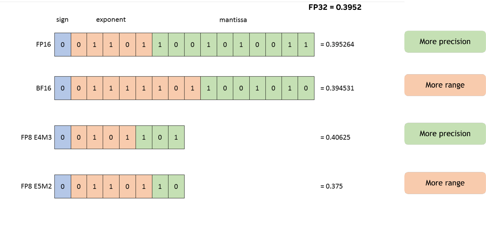
FP8 by itself is not a standardized format:
| Variant | Sign | Exponent | Mantissa | Best For | Dynamic Range | Precision |
|---|---|---|---|---|---|---|
| E4M3 | 1 | 4 | 3 | Weights & Activations (forward pass) | ~ ±448 | Higher |
| E5M2 | 1 | 5 | 2 | Gradients (backward pass) | ”~ ±57,000+ (wider)” | Lower |
Here is a comparison of the typical use cases and cost of using different precision variants:
| Format | Bits | Relative Memory | Speed Gain (vs FP32) | Typical Use Case | Accuracy Impact |
|---|---|---|---|---|---|
| FP32 | 32 | 1x | Baseline | Training (full precision) | Highest |
| FP16 | 16 | 0.5x | ~2x | Mixed training & inference | Small |
| FP8 | 8 | 0.25x | ~4x | Efficient training & inference | Moderate |
| FP4 | 4 | 0.125x | ~8x+ | Ultra-low bit inference | Higher (with scaling) |
FP16 is mature and safe, FP8 is the current sweet spot for many deployments, and FP4 represents the bleeding edge pushing toward even lower bits.
Quantizing Weights
For our NanoGPT model, we won’t see substantial benefits from quantizing weights because the model is so small (210k parameters). We may even see some slowdown when using a free Google Colab GPU since quantization adds its own overhead. However, it’s a good exercise to understand how it works.
Section 1: Baseline Benchmark
We want to measure first the FP32 inference latency and model size before touching anything.
import os, time, copy

def benchmark_generate(model, context, n_tokens=200, n_trials=5):
    """Returns mean latency in ms over n_trials runs."""
    model.eval()
    times = []
    with torch.no_grad():
        for _ in range(n_trials):
            t0 = time.perf_counter()
            model.generate(context, n_tokens)
            t1 = time.perf_counter()
            times.append((t1 - t0) * 1000)
    return sum(times) / len(times)

def model_size_mb(model):
    """Size of model parameters in MB."""
    total = sum(p.numel() * p.element_size() for p in model.parameters())
    return total / 1e6

context = torch.zeros((1, 1), dtype=torch.long, device=device)
fp32_ms  = benchmark_generate(model, context)
fp32_mb  = model_size_mb(model)
print(f"FP32 | size: {fp32_mb:.2f} MB | latency: {fp32_ms:.1f} ms")
The result we get is
FP32 | size: 0.84 MB | latency: 1292.2 ms
This means that our model is about 1MB in size and takes about 1.3 seconds to generate 200 tokens.
Section 2: Dynamic Quantization
For this section, we will quantize the linear layers of the model to INT8 precision.
We will start with the linear layers because that is where most of the parameters are stored. The LayerNorm is not touched because it is extremely sensitive to precision loss. The embedding table is not touched since they aren’t explicitly using matmul operations, thus there is no kernel that can speed it up.
The linear layer is where most of the weight matrices live, and compressing the size of the weights is what quantization serves to do.
import torch.quantization

model_dq = copy.deepcopy(model).cpu()
model_dq.eval()

devices = {p.device for p in model_dq.parameters()}
print("model_dq devices:", devices)  # should be {device(type='cpu')}

model_dq = torch.quantization.quantize_dynamic(
    model_dq,
    {nn.Linear},   # which layer types to quantize
    dtype=torch.qint8
)

print(model_dq.blocks[0].sa.proj)
print(model_dq.blocks[0].sa.proj.weight().dtype)

context_cpu = torch.zeros((1, 1), dtype=torch.long, device='cpu')  # CPU tensor
dq_ms  = benchmark_generate(model_dq, context_cpu)
dq_mb  = model_size_mb(model_dq)   # Note: may not reflect INT8 savings accurately
print(f"DQ INT8 | size: {dq_mb:.2f} MB | latency: {dq_ms:.1f} ms")


torch.manual_seed(42)
out = model_dq.generate(context_cpu, max_new_tokens=100)
print(decode(out[0].tolist()))  # Should still be Shakespeare-ish
Let’s walk through this step by step.
Deep copy to CPU. copy.deepcopy(model).cpu() creates an independent clone of the model and moves it to CPU. Dynamic quantization in PyTorch’s eager mode only supports CPU - the quantized INT8 kernels don’t have CUDA implementations. We call .eval() to disable dropout and set batch norm to inference mode.
Verify device placement. A quick sanity check that all parameters actually landed on CPU. If any tensor is still on CUDA, the quantization call below will silently produce wrong results or crash.
quantize_dynamic. This is the one-line API that does all the work. It walks the model, finds every nn.Linear layer, and replaces it with a DynamicQuantizedLinear. “Dynamic” means the weights are quantized to INT8 ahead of time (stored as INT8), but the activations are quantized on-the-fly at each forward pass using the actual min/max of the input tensor. This is simpler than static quantization (no calibration step needed) but slightly slower because it computes activation scales at runtime.
This function ideally should be used for Transformer like models, and RNN’s, or situations where you want quick quantization with minimal loss.
Every invocation, it does the following in order for the activations:
- Compute the min/max (or range) of the current activation tensor.
- Calculate the scale and zero-point for quantization.
- Quantize the floating-point activations to int8.
- Perform the quantized matrix multiplication (int8 GEMM).
- Dequantize the result back to floating point (so the next layer can use it).
Inspect a quantized layer. We print the first attention projection layer to confirm it’s now a DynamicQuantizedLinear, and verify the weight dtype is torch.qint8 - each weight value is stored as an 8-bit integer instead of a 32-bit float, a 4× memory reduction per parameter.
Benchmark. We create a CPU context tensor and measure latency and model size. Note that model_size_mb may undercount the savings - PyTorch stores quantized weights as packed INT8 tensors, but p.element_size() might report the unpacked size depending on the version.
Generate text. Finally, we seed the RNG and generate 100 tokens to verify the quantized model still produces coherent Shakespeare. The output won’t be identical to FP32 (quantization introduces small rounding errors), but it should be recognizably similar in quality.
The result we get is
model_dq devices: {device(type='cpu')}
DynamicQuantizedLinear(in_features=64, out_features=64, dtype=torch.qint8, qscheme=torch.per_tensor_affine)
torch.qint8
/tmp/ipykernel_2327/4228614202.py:9: DeprecationWarning: torch.ao.quantization is deprecated and will be removed in 2.10.
For migrations of users:
1. Eager mode quantization (torch.ao.quantization.quantize, torch.ao.quantization.quantize_dynamic), please migrate to use torchao eager mode quantize_ API instead
2. FX graph mode quantization (torch.ao.quantization.quantize_fx.prepare_fx,torch.ao.quantization.quantize_fx.convert_fx, please migrate to use torchao pt2e quantization API instead (prepare_pt2e, convert_pt2e)
3. pt2e quantization has been migrated to torchao (https://github.com/pytorch/ao/tree/main/torchao/quantization/pt2e)
see https://github.com/pytorch/ao/issues/2259 for more details
  model_dq = torch.quantization.quantize_dynamic(
DQ INT8 | size: 0.03 MB | latency: 1877.0 ms


KING LIf madam:
That is chard's to say, bening for yet are
Sed maks of qure of the maid thegnly so,
3 takeaways:
- The model shrank from 0.84 MB → 0.03 MB - a ~28× reduction. This makes sense: INT8 weights are 4× smaller than FP32, and PyTorch’s packed storage format compresses further.
- 1292 ms → 1877 ms, about 45% slower. This is counterintuitive but expected for a tiny model like NanoGPT (210k params). Dynamic quantization adds overhead per forward pass (computing activation min/max, quantizing inputs, dequantizing outputs), and for a model this small, that overhead dominates any benefit from cheaper INT8 matmuls.
- The generated text (“KING LIf madam: That is chard’s to say…”) is still recognizably Shakespeare-style, so the INT8 rounding errors didn’t destroy the model’s capabilities.
Section 3: Static (Post-Training) Quantization
This requires 3 steps fuse -> prepare -> calibrate -> convert
"""
Post-Training Static Quantization (Eager mode with QuantWrapper)

FX graph mode fails: Head.forward() has data-dependent control flow.
Broad QuantStub/DeQuantStub fails: attention bmm has no QuantizedCPU kernel.

Fix: wrap individual Linears with QuantWrapper so each does:
  float_in → quantize → int8_matmul → dequantize → float_out
Attention matmul stays in float.
"""
from torch.ao.quantization import QuantStub, DeQuantStub

class QuantWrapper(nn.Module):
    def __init__(self, module):
        super().__init__()
        self.quant = QuantStub()
        self.dequant = DeQuantStub()
        self.module = module
    def forward(self, x):
        return self.dequant(self.module(self.quant(x)))

model_sq = copy.deepcopy(model).cpu().eval()

# Disable the model-level QuantStub/DeQuantStub (too broad)
model_sq.quant = nn.Identity()
model_sq.dequant = nn.Identity()

for block in model_sq.blocks:
    torch.ao.quantization.fuse_modules(
        block.ffwd.net,
        [['0', '1']],   # net[0]=Linear, net[1]=ReLU → fused LinearReLU
        inplace=True
    )

qcfg = torch.ao.quantization.get_default_qconfig('fbgemm')
model_sq.qconfig = None  # nothing quantized by default

# Wrap every Linear we want statically quantized
for block in model_sq.blocks:
    # FFN
    block.ffwd.net[0] = QuantWrapper(block.ffwd.net[0]); block.ffwd.net[0].qconfig = qcfg
    block.ffwd.net[2] = QuantWrapper(block.ffwd.net[2]); block.ffwd.net[2].qconfig = qcfg
    # Attention projection
    block.sa.proj = QuantWrapper(block.sa.proj); block.sa.proj.qconfig = qcfg
    # K/Q/V projections (output is dequanted → attention matmul stays float)
    for head in block.sa.heads:
        head.key   = QuantWrapper(head.key);   head.key.qconfig   = qcfg
        head.query = QuantWrapper(head.query); head.query.qconfig = qcfg
        head.value = QuantWrapper(head.value); head.value.qconfig = qcfg

model_sq.lm_head = QuantWrapper(model_sq.lm_head); model_sq.lm_head.qconfig = qcfg

torch.ao.quantization.prepare(model_sq, inplace=True)
print("Prepared for calibration (observers inserted)")
Let’s break this down step by step.
The problem. PyTorch’s static quantization needs QuantStub and DeQuantStub markers to know where to convert between float and INT8. If you place them at the model level (wrapping the entire forward pass), the attention bmm operation breaks - there’s no QuantizedCPU kernel for batched matrix multiplication. FX graph mode doesn’t work either because our Head.forward() has data-dependent control flow (the if past_kvs branch). The fix is to wrap each Linear layer individually so quantization happens at the boundary of each matmul, while attention stays in float.
QuantWrapper. This is a thin nn.Module that sandwiches any layer between a QuantStub and DeQuantStub. On the forward pass, the float input gets quantized to INT8, passes through the wrapped module’s INT8 kernel, and the output gets dequantized back to float. This means each wrapped Linear does float → int8 → matmul → int8 → float, while everything between (like attention’s bmm) stays in float.
Deep copy and disable model-level stubs. We deep copy the model to CPU (static quantization only works on CPU in eager mode) and replace the model-level QuantStub/DeQuantStub with nn.Identity() - since we’re doing per-layer wrapping instead.
Fuse Linear + ReLU. For each transformer block, we fuse net[0] (Linear) and net[1] (ReLU) in the feedforward network into a single LinearReLU module. Fusing lets the quantized kernel apply ReLU directly on the INT8 output without an intermediate dequantize-requantize round trip, which is both faster and more accurate.
Set qconfig. We grab the default quantization config for the fbgemm backend (Intel x86 optimized INT8 kernels). Setting model_sq.qconfig = None means nothing is quantized by default - we’ll opt in layer by layer.
Wrap every Linear. For each transformer block, we wrap the feedforward layers (net[0] the fused LinearReLU, net[2] the second Linear), the attention output projection (sa.proj), and each head’s key, query, and value projections. Each wrapped module gets assigned the qcfg so PyTorch knows it should be quantized. The final lm_head (the output projection from hidden dim to vocabulary size) is also wrapped.
Prepare for calibration. torch.ao.quantization.prepare() walks the model and inserts observer modules at every QuantStub. Observers record the min/max activation ranges during calibration (the next step), which PyTorch uses to compute optimal scale and zero-point values for INT8 quantization.
Section 3.1: Calibration
# Calibration
model_sq.eval()
with torch.no_grad():
    for _ in range(100):
        xb, _ = get_batch('val')
        model_sq(xb.cpu())

torch.ao.quantization.convert(model_sq, inplace=True)
print("Converted to quantized model")
print(model_sq.blocks[0].sa.proj.module)  # should show QuantizedLinear

context_cpu = torch.zeros((1, 1), dtype=torch.long, device='cpu')
sq_ms = benchmark_generate(model_sq, context_cpu)
sq_mb = model_size_mb(model_sq)
print(f"SQ INT8 | size: {sq_mb:.2f} MB | latency: {sq_ms:.1f} ms")
Calibration. We run 100 batches of validation data through the model. The inserted observers record the min/max activation values for each wrapped layer. This “burn-in” period is crucial: without it, the observers would see only zeros or outliers, leading to poor quantization scales and degraded accuracy.
Convert. torch.ao.quantization.convert() finalizes the quantization. It uses the observed min/max ranges to compute optimal scale and zero-point values for each layer, then replaces the QuantStub/DeQuantStub wrappers with actual quantized linear modules (QuantizedLinear).
Verify. We print the first attention projection layer to confirm it’s now a QuantizedLinear with computed scale and zero-point. The qscheme=torch.per_channel_affine indicates per-channel quantization (different scale/zero-point per output channel), which is more accurate than per-tensor.
Benchmark. We measure latency and size again. You’ll notice the size is identical to dynamic quantization (0.03 MB) - both use INT8 weights. The latency, however, is now ~2353 ms, slower than dynamic quantization’s ~1877 ms. This slowdown isn’t from the calibration phase, but rather the per-layer QuantWrapper overhead during inference (converting back and forth between float and INT8 at every layer), which dominates the execution time for very small models.
Here is the result:
/tmp/ipykernel_2327/2224656562.py:8: DeprecationWarning: torch.ao.quantization is deprecated and will be removed in 2.10.
For migrations of users:
1. Eager mode quantization (torch.ao.quantization.quantize, torch.ao.quantization.quantize_dynamic), please migrate to use torchao eager mode quantize_ API instead
2. FX graph mode quantization (torch.ao.quantization.quantize_fx.prepare_fx,torch.ao.quantization.quantize_fx.convert_fx, please migrate to use torchao pt2e quantization API instead (prepare_pt2e, convert_pt2e)
3. pt2e quantization has been migrated to torchao (https://github.com/pytorch/ao/tree/main/torchao/quantization/pt2e)
see https://github.com/pytorch/ao/issues/2259 for more details
  torch.ao.quantization.convert(model_sq, inplace=True)
Converted to quantized model
QuantizedLinear(in_features=64, out_features=64, scale=0.011876680888235569, zero_point=65, qscheme=torch.per_channel_affine)
SQ INT8 | size: 0.03 MB | latency: 2353.2 ms
The result confirms the conversion worked - the projection layer is now a QuantizedLinear with per_channel_affine quantization, meaning each of the 64 output channels has its own scale and zero-point (the printed scale=0.0119, zero_point=65 are for one representative channel). This is more precise than dynamic quantization’s per_tensor_affine scheme, where a single scale covers the entire weight matrix - per-channel avoids the problem where one outlier channel forces a wide range that wastes precision for all the others.
The size is identical to dynamic quantization at 0.03 MB - both approaches store INT8 weights, so the compression ratio is the same. The latency, however, is the worst of all three approaches at 2353 ms (FP32: 1292 ms, dynamic: 1877 ms). This is the cost of our QuantWrapper approach: every wrapped Linear performs a float → quantize → int8_matmul → dequantize → float round trip, and with 6 wrapped layers per transformer block (K, Q, V, proj, two FFN linears) plus lm_head, that’s a lot of quantize/dequantize overhead for a model where the actual matmuls take microseconds. In production systems with large models, this overhead is negligible compared to the massive INT8 matmul savings - but for our 210k-parameter NanoGPT, it dominates.
Here is the final comparison:
Method                Size (MB)   Latency (ms)    Speedup
--------------------------------------------------------
FP32 (baseline)            0.84         1292.2      1.00x
Dynamic INT8               0.03         1877.0      0.69x
Static INT8                0.03         2353.2      0.55x
We can see that both quantization methods achieve a massive 28× memory reduction (0.84 MB → 0.03 MB), but neither delivers a speed improvement - in fact, both are slower than the FP32 baseline. This is the key lesson: quantization’s latency benefit comes from replacing expensive FP32 matrix multiplications with cheaper INT8 ones, but our NanoGPT model has only 210k parameters, so the matmuls themselves take microseconds. The fixed overhead of quantization (computing scales, packing/unpacking INT8 tensors, dequantizing outputs) dwarfs those microsecond matmuls, resulting in a net slowdown.
Dynamic quantization (0.69×) beats static (0.55×) on latency because it has less per-layer overhead - there’s no QuantStub/DeQuantStub wrapper around every Linear, just a single quantize_dynamic call that swaps in optimized DynamicQuantizedLinear modules. Static quantization pays for higher accuracy (per-channel scales from calibration) with more conversion overhead at every layer boundary.
In production, with models like LLaMA-70B where a single forward pass involves billions of multiply-accumulate operations, the INT8 compute savings overwhelm the fixed overhead and you’d see the expected 2-4× speedup. For our tiny model, the takeaway is simpler: quantization is a memory optimization first. If your goal is to fit a model into limited VRAM or ship a smaller binary, quantization delivers immediately. The speed benefit is a bonus that only kicks in at scale.
You can find the entire source code here: https://github.com/czhou578/multimodal-inference-visualizer/blob/main/nanogpt-static-quant.ipynb
CZ