Comparing NanoGPT vs SGLang
RadixAttention was the reason I built the radix tree in the first place. SGLang’s original paper introduced the idea of using a radix tree to manage KV cache sharing across requests, and I wanted to understand it from the ground up by implementing it myself in NanoGPT.
Now that I’ve done that, I went back and read SGLang’s actual radix_cache.py - all ~800 lines of it - to see how the production version compares. The experience was humbling. The core algorithm is the same: compressed trie, prefix matching, node splitting. But SGLang makes a handful of non-obvious design choices that completely change the performance characteristics, and I want to walk through the ones that surprised me most.
The shape of the two systems
Here are the two stacks, top to bottom:
SGLang’s Radix Cache Stack
┌─────────────────────────────────────────────┐
│  RadixCache (radix_cache.py)                │ ← Top-level API
│    Extends BasePrefixCache + KVCacheEvents  │
├─────────────────────────────────────────────┤
│  TreeNode                                    │ ← Node metadata
│    children, key, value, lock_ref,           │
│    hit_count, priority, host_value           │
├─────────────────────────────────────────────┤
│  RadixKey                                    │ ← Edge label abstraction
│    token_ids, extra_key, bigram mode         │
│    Exponential-search matching               │
├─────────────────────────────────────────────┤
│  token_to_kv_pool_allocator                  │ ← Physical KV memory pool
│    Alloc/free of KV cache indices            │
├─────────────────────────────────────────────┤
│  evictable_leaves (set)                      │ ← Leaf-first LRU eviction
│    Priority-aware heap eviction              │
└─────────────────────────────────────────────┘
NanoGPT’s Radix Tree Stack
┌─────────────────────────────────────────────┐
│  RadixTree (nanogpt-radix-tree-.py)         │ ← Top-level API
│    match_prefix, insert, eviction            │
├─────────────────────────────────────────────┤
│  RadixNode                                   │ ← Node metadata
│    children, token_ids, kv_data, lock_ref    │
├─────────────────────────────────────────────┤
│  Per-request KV cache (dict)                 │ ← KV data on request
│    kv_cache[(layer, head)] = (k, v)          │
└─────────────────────────────────────────────┘
SGLang has five layers. We have three. But the biggest difference is hiding in the node objects - and it’s the same lesson as the vLLM comparison.
The node tells you everything
Let’s start by looking at what lives on a single tree node, because that one design decision radiates through every other part of the system.
SGLang’s TreeNode:
class TreeNode:
    counter = 0

    def __init__(self, id=None, priority=0):
        self.children = defaultdict(TreeNode)
        self.parent: TreeNode = None
        self.key: RadixKey = None
        self.value: Optional[torch.Tensor] = None   # KV cache indices (int64)
        self.lock_ref = 0
        self.last_access_time = time.monotonic()
        self.creation_time = time.monotonic()
        self.hit_count = 0
        self.host_ref_counter = 0                    # CPU offload lock
        self.host_value: Optional[torch.Tensor] = None
        self.hash_value: Optional[List[str]] = None  # per-page SHA256
        self.priority = priority                     # priority-aware eviction
        self.id = TreeNode.counter
Our RadixNode:
class RadixNode:
    def __init__(self):
        self.children: Dict[int, RadixNode] = {}
        self.parent: Optional[RadixNode] = None
        self.token_ids: Tuple[int, ...] = ()
        self.kv_data: Optional[Dict] = None   # actual KV tensors stored here
        self.lock_ref: int = 0
        self.last_access_time: int = 0
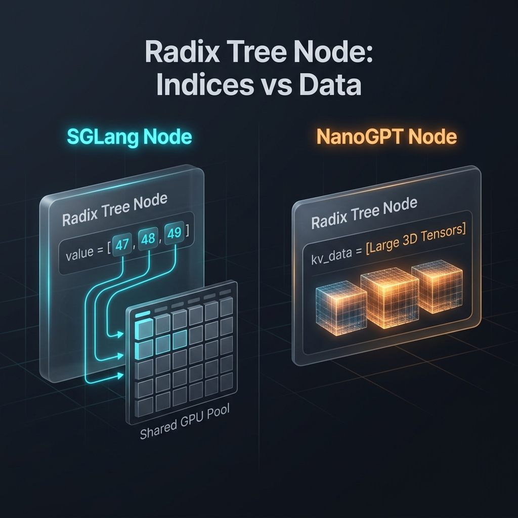
The field that matters most is value vs kv_data. SGLang’s value is a 1D torch.int64 tensor - a list of indices into a shared GPU memory pool. The actual KV tensors live elsewhere, pre-allocated on the GPU. The node just says “my KV data is at pool slots [47, 48, 49, 50].” Our kv_data is a dict of actual KV tensors, stored right on the node.
This sounds like a minor detail. It isn’t.
| Feature | SGLang | NanoGPT |
|---|---|---|
| KV data storage | value = torch.Tensor of indices into a shared GPU memory pool |
kv_data = dict of actual KV tensors stored on the node |
| Edge label | RadixKey object (supports bigram, extra_key, page alignment) |
Raw tuple[int, ...] |
| Children dict | defaultdict(TreeNode) - auto-creates on access |
Dict[int, RadixNode] - standard dict |
| Access tracking | time.monotonic() - real wall-clock time |
Integer step counter |
| Hit counting | hit_count - tracks how often a node is matched |
Not implemented |
| Priority | Per-node priority for priority-aware eviction |
Not implemented |
| Host offload | host_value + host_ref_counter for CPU ↔ GPU tiering |
Not implemented |
When a request in SGLang matches a prefix, it gets back those indices and uses them directly - no copying. Two requests sharing a 200-token prefix point to the same 200 pool slots. Zero additional GPU memory.
When a request in NanoGPT matches a prefix, load_from_radix_tree() clones every (layer, head) tensor pair onto the request’s private cache. Two requests sharing a 200-token prefix? That’s 2× the memory. Same pattern we saw in the vLLM comparison - the “indices vs data” design decision ripples through everything downstream.
Edge labels are not just labels
This is something I didn’t appreciate until I read SGLang’s code. In our implementation, an edge is just tuple[int, ...] - a sequence of token IDs. In SGLang, it’s a full RadixKey object:
class RadixKey:
    __slots__ = ("token_ids", "extra_key", "is_bigram")

    def __init__(self, token_ids: array[int], extra_key=None, is_bigram=False):
        self.token_ids = token_ids     # array('q', [...]) - compact C array
        self.extra_key = extra_key     # LoRA ID, cache salt, etc.
        self.is_bigram = is_bigram     # EAGLE speculative decoding mode

    def match(self, other, page_size=1) -> int:
        # Exponential search + binary search for divergence point
        # O(log(prefix_len)) C-level slice comparisons
        ...
Three things stand out:
First, token_ids is a C-level array('q', ...), not a Python tuple. This matters because RadixKey.match() compares slices of these arrays using C-level equality checks (t0[lo:hi] != t1[lo:hi]), which avoids per-token Python iteration.
Second, extra_key enables namespace isolation. If you’re serving multiple LoRA adapters or using cache salts for security isolation, two sequences with the same tokens but different extra_key values don’t share cache. We don’t support this at all.
Third, the matching algorithm itself. SGLang uses exponential search: start comparing 1 token, then 2, then 4, then 8, doubling each time. The moment a comparison fails, binary-search within that window to find the exact divergence point. For an edge with 1,000 matching tokens, that’s ~10 C-level slice comparisons (exponential galloping) plus ~10 more (binary search) - roughly 20 operations total. We do 1,000 Python iterations. The asymptotic difference is O(log n) vs O(n), but the constant-factor difference is even bigger because SGLang never enters a Python for loop at all.
| Feature | SGLang | NanoGPT |
|---|---|---|
| Data type | array('q', ...) - C-level int64 array |
Python tuple[int, ...] |
| Matching algorithm | Exponential search + binary search - O(log n) slice compares | Linear scan - O(n) per-token Python loop |
| Page alignment | page_aligned(page_size) truncates to page boundary |
Manual (matched // block_size) * block_size |
| Namespace isolation | extra_key separates LoRA adapters, cache salts |
Not supported |
| Bigram mode | is_bigram=True for EAGLE speculative decoding |
Not supported |
Prefix matching: same algorithm, different guts
The prefix matching walk is structurally identical in both systems. You start at the root, look up the first token in children, compare the edge, split if needed, and continue. Here they are side by side:
# SGLang
def _match_prefix_helper(self, node, key):
    access_time = time.monotonic()
    node.last_access_time = access_time
    child_key = key.child_key(self.page_size)

    value = []
    while len(key) > 0 and child_key in node.children.keys():
        child = node.children[child_key]
        child.last_access_time = access_time
        prefix_len = child.key.match(key, page_size=self.page_size)
        if prefix_len < len(child.key):
            new_node = self._split_node(child.key, child, prefix_len)
            value.append(new_node.value)
            node = new_node
            break
        else:
            value.append(child.value)
            node = child
            key = key[prefix_len:]
            if len(key):
                child_key = key.child_key(self.page_size)
    return value, node
# NanoGPT
def match_prefix(self, token_ids):
    node = self.root
    matched = 0
    while matched < len(token_ids):
        next_token = token_ids[matched]
        child = node.children.get(next_token)
        if child is None: break

        edge_tokens = child.token_ids
        edge_match_len = 0
        while (edge_match_len < len(edge_tokens) and
               matched + edge_match_len < len(token_ids) and
               edge_tokens[edge_match_len] == token_ids[matched + edge_match_len]):
            edge_match_len += 1

        if edge_match_len < len(edge_tokens):
            child = self._split_node(child, edge_match_len)
            matched += edge_match_len
            node = child
            break

        matched += edge_match_len
        node = child
    return node, matched
Squint at these and they’re the same function. Walk down, compare edges, split on partial match, advance. The differences:
- SGLang returns KV indices directly (
valuelist) - the caller can hand these straight to the GPU kernel. We return a(node, match_count)pair that the caller has to walk to extract KV data. - SGLang updates
last_access_timeon every traversed node during the match. We don’t - our access times only update during lock/unlock. - SGLang uses
RadixKey.match()(exponential search) for edge comparison. We use a per-tokenwhileloop.
| Feature | SGLang | NanoGPT |
|---|---|---|
| Return value | (List[torch.Tensor], TreeNode) - concatenated KV indices + last node |
(RadixNode, int) - last node + match count |
| Edge matching | RadixKey.match() - exponential search |
Per-token while loop |
| Access time update | time.monotonic() on every traversed node |
Not updated during match |
| Split on partial match | Yes - identical logic | Yes - identical logic |
Node splitting: where “indices vs data” really bites
Splitting is the trickiest operation on a radix tree. When a new sequence partially matches an existing edge, you have to cut the edge in two, create a new intermediate node, and re-wire all the parent/child pointers. The logic is the same in both systems. But the cost is wildly different.
SGLang:
def _split_node(self, key, child, split_len):
    new_node = TreeNode(priority=child.priority)
    new_node.hit_count = child.hit_count
    new_node.children = {key[split_len:].child_key(self.page_size): child}
    new_node.parent = child.parent
    new_node.lock_ref = child.lock_ref
    new_node.key = child.key[:split_len]
    new_node.value = child.value[:split_len].clone()
    child.parent = new_node
    child.key = child.key[split_len:]
    child.value = child.value[split_len:].clone()
    new_node.parent.children[key.child_key(self.page_size)] = new_node
    return new_node
NanoGPT:
def _split_node(self, child, split_len):
    new_mid = RadixNode()
    new_mid.token_ids = child.token_ids[:split_len]
    new_mid.parent = child.parent
    new_mid.last_access_time = child.last_access_time
    new_mid.lock_ref = child.lock_ref

    if child.kv_data is not None:
        new_mid.kv_data = {}
        new_child_kv = {}
        for (layer, head), (k, v) in child.kv_data.items():
            new_mid.kv_data[(layer, head)] = (
                k[:, :split_len, :].clone(), v[:, :split_len, :].clone()
            )
            new_child_kv[(layer, head)] = (
                k[:, split_len:, :].clone(), v[:, split_len:, :].clone()
            )
        child.kv_data = new_child_kv

    child.token_ids = child.token_ids[split_len:]
    child.parent = new_mid
    new_mid.children[child.token_ids[0]] = child
    new_mid.parent.children[new_mid.token_ids[0]] = new_mid
    return new_mid
See the difference? SGLang’s split clones a 1D int64 tensor - one value[:split_len].clone() call. That’s it. It’s slicing a list of pool indices.
Our split has to iterate over every (layer, head) pair and clone 3D KV tensors for both halves. For a model with 6 layers and 6 heads, that’s 72 tensor allocations (36 for the new mid-node, 36 for the truncated child). For a production model with 80 layers and 128 heads? You don’t want to think about it.
| Feature | SGLang | NanoGPT |
|---|---|---|
| Value split | value[:split_len].clone() - slicing a 1D index tensor |
Per-(layer, head) 3D tensor slicing + clone |
| Cost | O(split_len) - single tensor clone | O(n_layer × n_head × split_len) - many tensor clones |
| Hash split | split_node_hash_value() preserves per-page hashes |
Not applicable |
This is the single most convincing argument for the “indices not data” design. Every tree mutation - split, insert, evict - becomes dramatically cheaper when you’re manipulating a list of integers instead of actual tensor data.
Eviction: surgical precision vs no eviction at all

This is the section where the two systems diverge the most. SGLang has a full eviction subsystem. NanoGPT doesn’t have tree-level eviction at all.
# SGLang
def evict(self, params: EvictParams):
    leaves = list(self.evictable_leaves)
    eviction_heap = [
        (self.eviction_strategy.get_priority(node), node) for node in leaves
    ]
    heapq.heapify(eviction_heap)

    num_evicted = 0
    while num_evicted < num_tokens and len(eviction_heap):
        _priority, x = heapq.heappop(eviction_heap)
        self.token_to_kv_pool_allocator.free(x.value)
        num_evicted += len(x.value)
        self._delete_leaf(x)

        # Parent may become a new leaf
        if len(x.parent.children) == 0 and x.parent.lock_ref == 0:
            heapq.heappush(eviction_heap, (new_priority, x.parent))
SGLang maintains a set of evictable_leaves - nodes that are leaves and have lock_ref == 0. When the allocator runs out of memory, evict() builds a min-heap of these leaves by priority, pops the lowest-priority leaf, frees its KV indices back to the pool, and deletes it from the tree. If the parent becomes childless and unlocked, it cascades into a new evictable leaf and gets pushed onto the heap.
This is beautiful. You can surgically reclaim memory from unused suffixes while keeping shared prefixes intact. If 8 requests branched from the same system prompt and 7 of them have finished, the 7 leaf nodes get evicted but the shared trunk stays. The 8th request is unaffected.
NanoGPT? Our tree just grows. Nodes are never deleted. Memory management happens at the request level - the scheduler’s _maybe_preempt() kicks out entire requests when KV token count exceeds a threshold. If a tree node holds actual tensor data (and ours do), that memory is pinned until the process exits. This was a deliberate simplification, but it means our tree is really a write-only cache, not a managed memory structure.
| Feature | SGLang | NanoGPT |
|---|---|---|
| Eviction granularity | Per-node (leaf-first) | Per-request (whole request preempted) |
| Eviction trigger | evict(num_tokens) called when allocator runs out |
_maybe_preempt() when KV tokens > threshold |
| Eviction strategy | Pluggable (lru, priority, custom) via eviction_strategy |
Not applicable at tree level |
| Leaf tracking | evictable_leaves: set - maintained incrementally |
Not tracked |
| Parent cascading | After deleting leaf, parent may become new evictable leaf | Not applicable |
| Locked nodes | lock_ref > 0 prevents eviction |
lock_ref > 0 prevents eviction (but at request level) |
Lock reference counting: same idea, different bookkeeping
Both systems use the same fundamental mechanism to prevent eviction of nodes that are actively in use: walk from the matched node up to the root, incrementing lock_ref on each node. When the request finishes, walk back down and decrement. A node with lock_ref > 0 can never be evicted.
# SGLang
def inc_lock_ref(self, node):
    delta = 0
    while node != self.root_node:
        if node.lock_ref == 0:
            self.evictable_size_ -= len(node.key)
            self.protected_size_ += len(node.key)
        node.lock_ref += 1
        self._update_leaf_status(node)
        node = node.parent
    return IncLockRefResult(delta=delta)
# NanoGPT
for pnode in prefix_path:
    pnode.lock_ref += 1
Same walk. But SGLang does two extra things on every lock transition: it updates evictable_size_ / protected_size_ (so the system always knows how much memory is reclaimable vs pinned), and it calls _update_leaf_status() to maintain the evictable_leaves set. These are the bookkeeping costs of having a real eviction system.
Our version is four lines. The tradeoff: we don’t know how much memory is evictable at any given time because we don’t track it.
| Feature | SGLang | NanoGPT |
|---|---|---|
| Walk direction | Leaf → root (same) | Leaf → root (same) |
| Size accounting | evictable_size_ / protected_size_ updated on transitions |
Not tracked |
| Leaf status | _update_leaf_status() maintains evictable set |
Not tracked |
| Path storage | Stored on req.last_node - only the leaf, walks up |
Stored on request._radix_path - entire path list |
Insertion: one pass vs two passes
SGLang inserts in a single iterative walk - it walks the existing prefix, splitting where necessary, and only creates a new node for the truly new suffix. Along the way it increments hit counts, propagates priorities, tracks evictable sizes, and deduplicates KV indices.
# SGLang
def _insert_helper(self, node, key, value, priority=0, chunked=False):
    while len(key) > 0 and child_key in node.children.keys():
        node = node.children[child_key]
        prefix_len = node.key.match(key, page_size=self.page_size)
        total_prefix_length += prefix_len
        key = key[prefix_len:]
        value = value[prefix_len:]
        if prefix_len < len(node.key):
            new_node = self._split_node(node.key, node, prefix_len)
            node = new_node
        ...
    if len(key):
        new_node = TreeNode(priority=priority)
        new_node.parent = node
        new_node.key = key
        new_node.value = value.clone()
        node.children[child_key] = new_node
        self.evictable_size_ += len(key)
        self._update_leaf_status(node)
        self._update_leaf_status(new_node)
    return total_prefix_length
We do it in two phases: match_prefix() first (which might split), then append the remainder:
# NanoGPT
def insert(self, token_ids, kv_data_full, block_size):
    node, matched = self.match_prefix(token_ids)
    if matched == len(token_ids): return

    remaining = token_ids[matched:]
    new_node = RadixNode()
    new_node.token_ids = tuple(remaining)
    new_node.parent = node

    new_node.kv_data = {}
    for (layer, head), (k, v) in kv_data_full.items():
        new_node.kv_data[(layer, head)] = (
            k[:, matched:matched + len(remaining)].clone(),
            v[:, matched:matched + len(remaining)].clone(),
        )
    node.children[remaining[0]] = new_node
Our two-phase approach is cleaner to read, but it can’t update metadata along the existing prefix path (no hit count bumps, no priority propagation) and it can’t deduplicate indices mid-insertion the way SGLang does.
Request lifecycle: automatic vs manual
The last difference is in how the tree integrates with the rest of the system. SGLang has dedicated methods for both finished and unfinished requests:
cache_finished_req()- inserts the full sequence (prompt + output) into the tree, frees duplicate indices, decrements lockscache_unfinished_req()- inserts partial progress (chunked prefill), re-matches to get updated indices, transfers locks
NanoGPT does this manually in the generation loop:
# On prefill completion:
insert_into_radix_tree(prefill_req, scheduler.radix_tree, scheduler.block_size)
scheduler.radix_tree.unlock_radix_path(prefill_req)

# On request completion:
scheduler.radix_tree.unlock_radix_path(req)
SGLang’s cache_unfinished_req() is particularly interesting - it handles the case where a request is mid-prefill and the tree has been modified by other requests since the last step. It re-matches the prefix, transfers lock references from the old node to the new one, and adjusts KV indices. We don’t handle this at all; we only insert into the tree when prefill is fully complete.
| Feature | SGLang | NanoGPT |
|---|---|---|
| Finished request caching | cache_finished_req() - handles dedup, index transfer, lock release |
insert_into_radix_tree() - manual call in loop |
| Unfinished request caching | cache_unfinished_req() - incremental caching during chunked prefill |
Not implemented - only inserts on prefill completion |
| Index deduplication | Frees indices that were already in tree | Not applicable (copies data, doesn’t share indices) |
| Lock transfer | dec_lock_ref(old_node) → inc_lock_ref(new_node) atomically |
Manual lock/unlock at separate points |
What NanoGPT captures vs what production requires
| Concept | NanoGPT | SGLang | Notes |
|---|---|---|---|
| Radix tree structure | ✅ | ✅ | Identical trie with compressed edges |
| Prefix matching with split | ✅ | ✅ | Same algorithm |
| Node splitting | ✅ | ✅ | Same logic, different cost |
| Lock reference counting | ✅ (simple) | ✅ (with size tracking) | Same walk-to-root pattern |
| KV sharing via indices | ❌ (copies data) | ✅ (shared indices) | SGLang’s memory advantage |
| Leaf-first eviction | ❌ | ✅ | Critical for memory management |
| Evictable leaf tracking | ❌ | ✅ (incremental set) | Enables O(1) leaf discovery |
| Priority-aware eviction | ❌ | ✅ (pluggable strategy) | Production scheduling |
| Page-aligned operations | ❌ (manual) | ✅ (page_size parameter) |
GPU memory alignment |
| Exponential-search matching | ❌ (linear scan) | ✅ | Performance at scale |
| Bigram mode (EAGLE) | ❌ | ✅ | Speculative decoding support |
| LoRA / cache salt isolation | ❌ | ✅ (extra_key) |
Multi-tenant serving |
| Host ↔ device tiering | ❌ | ✅ (host_value) |
HiCache CPU offloading |
| Chunked prefill caching | ❌ | ✅ (cache_unfinished_req) |
Incremental caching |
What I took away from this
The three biggest differences between our radix tree and SGLang’s all trace back to the same root cause: what the node holds.
1. Indices vs data. SGLang’s tree nodes store a 1D int64 tensor of pool indices. Splitting a node is one tensor slice. Matching a prefix returns indices the GPU can use directly. Sharing a prefix costs zero additional memory. Our nodes store the actual KV tensors, so splitting is O(n_layer × n_head) tensor allocations, matching requires cloning data onto each request, and sharing duplicates everything. One field, cascading consequences.
2. Fine-grained eviction vs none. Because SGLang’s nodes hold lightweight indices, evicting a leaf means freeing a handful of integers back to the allocator - fast and surgical. Our nodes hold heavy tensor data, so we punted on tree-level eviction entirely. Memory management happens at the request level (preempt the whole request), which is a much blunter instrument. SGLang can trim individual unused suffixes; we can only kill entire requests.
3. Exponential-search matching. SGLang’s RadixKey.match() avoids per-token Python iteration by comparing array slices in C, galloping in doubling windows. For an edge with 1,000 matching tokens, SGLang does ~20 C-level slice comparisons. We do 1,000 Python iterations. In multi-turn conversations where shared prefixes can be thousands of tokens long, this is a significant performance difference.
The pattern is the same one I saw in vLLM: the educational implementation makes the obvious choice at each fork (store data directly, skip eviction, use a Python loop), and those choices compose into a system that works but doesn’t scale. The production system makes the non-obvious choice (indirection through indices, leaf-set tracking, exponential search), and those choices compose into something that handles real workloads.
Building the simple version first was the right call. It gave me the vocabulary to understand why every “weird” decision in SGLang’s code exists.
CZ