NanoGPT: Fused Multi-Head Attention
In the KV cache post, each attention head was its own nn.Module - a separate Head class with its own nn.Linear layers for query, key, and value projections. A MultiHeadAttention wrapper held a ModuleList of these heads, ran each one independently, and concatenated the results. This is clean and pedagogically useful: you can read one head in isolation and understand exactly what self-attention does. But no production model works this way.
The problem is that each head launches its own matrix multiplication. With 4 heads, that’s 12 separate linear projections per attention layer (4 queries + 4 keys + 4 values), each one dispatching its own CUDA kernel. The overhead of scheduling all those kernel launches dominates the actual compute, especially at small dimensions. And the separate nn.Linear layers mean the weights live in different memory allocations, so the GPU can’t coalesce them into a single efficient read.
The fix is fused multi-head attention: replace the per-head projections with a single nn.Linear(n_embd, 3 * n_embd) that computes Q, K, and V for all heads in one shot. One kernel launch, one weight matrix, one memory read. Then you just reshape the output to separate the heads.
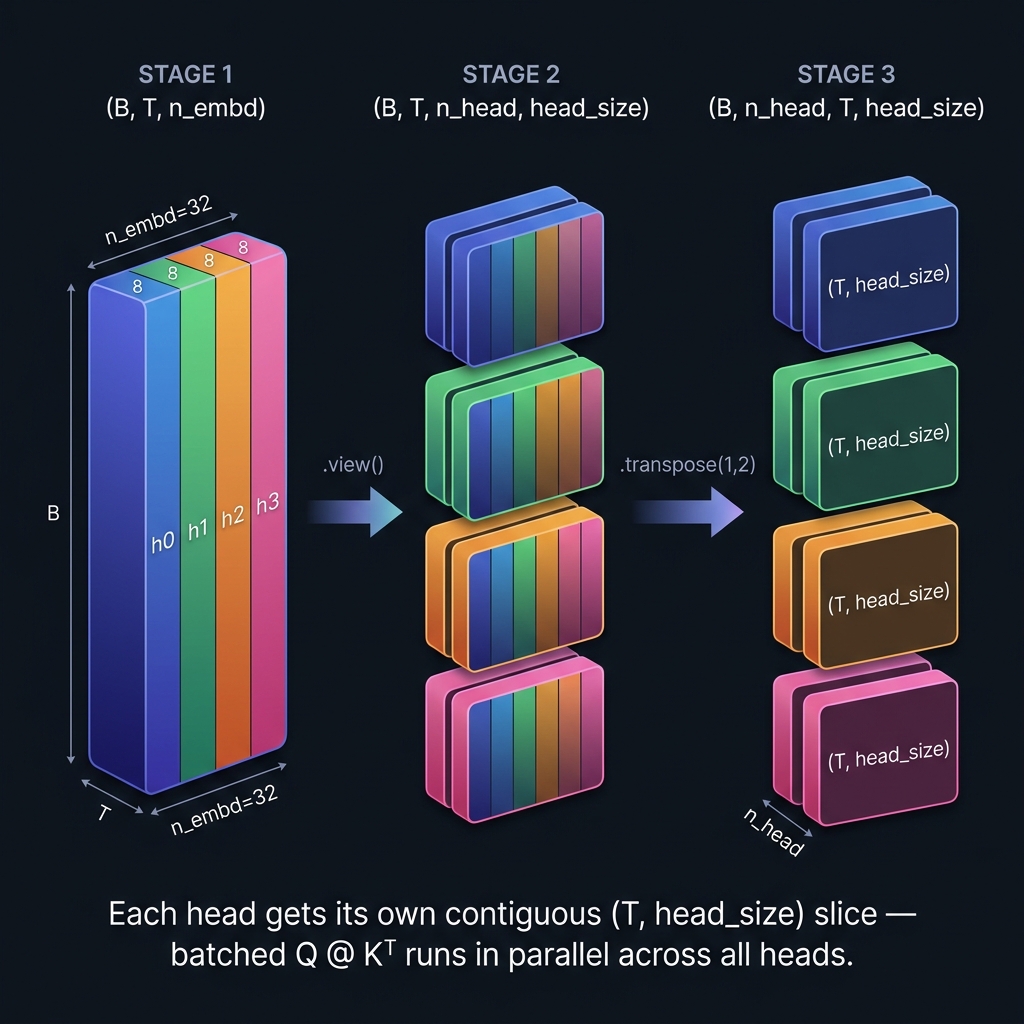
This sounds trivial but the reshape is where everyone gets confused, including me. The tensor gymnastics to go from a flat (B, T, n_embd) output to the (B, n_head, T, head_size) layout that batched attention needs are subtle enough that it’s worth walking through them carefully.
The fused QKV projection
Here’s the old architecture and the new one, side by side:
OLD (per-head):                    NEW (fused):
┌─────────────────────┐            ┌─────────────────────────┐
│ Head 0              │            │ CausalSelfAttention      │
│   q = Linear(32→8)  │            │   qkv = Linear(32→96)   │
│   k = Linear(32→8)  │   ──►     │   attn_proj = Linear(32→32) │
│   v = Linear(32→8)  │            │                          │
├─────────────────────┤            │   One class, one forward │
│ Head 1              │            │   pass, all heads fused   │
│   q = Linear(32→8)  │            └─────────────────────────┘
│   k = Linear(32→8)  │
│   v = Linear(32→8)  │
├─────────────────────┤
│ Head 2, Head 3 ...  │
└─────────────────────┘

12 separate nn.Linear         →    1 fused nn.Linear
12 kernel launches per layer  →    1 kernel launch
The fused linear projects every token into a 3 * n_embd-dimensional vector - three copies of n_embd packed side by side, one for Q, one for K, one for V. With our hyperparameters (n_embd=32, n_head=4, head_size=8), that’s 3 * 32 = 96 values per token.
class CausalSelfAttention(nn.Module):
    """
    Implement self-attention with fused QKV projection and KV cache.
    """
    def __init__(self, num_heads, head_size):
        super().__init__()
        self.qkv = nn.Linear(n_embd, 3 * n_embd, bias=False)
        self.attn_proj = nn.Linear(n_embd, n_embd)
        self.num_heads = num_heads
        self.head_size = head_size
        self.register_buffer('tril', torch.tril(torch.ones(block_size, block_size)))

        self.key_cache = None
        self.value_cache = None
Two things to note. First, self.qkv has a weight matrix of shape (96, 32) - it maps the 32-dimensional input into a 96-dimensional output where the first 32 values are Q, the next 32 are K, and the last 32 are V. This is equivalent to running three separate nn.Linear(32, 32) layers and concatenating the results, but in one matmul. Second, self.attn_proj is the output projection - the linear layer that maps the attention output back to n_embd dimensions. In the old architecture, this was implicit in the MultiHeadAttention.proj layer that came after concatenation. Here it’s explicit.
The reshape: why .view() then .transpose()
This is the part that tripped me up. After the fused projection, we have tensors of shape (B, T, n_embd) - a flat 32-wide vector per token. But attention needs (B, n_head, T, head_size) - each head working independently on its own (T, head_size) slice. How do we get there?
def forward(self, x):
    B, T, C = x.shape
    qkv = self.qkv(x) # (B, T, 3 * n_embd) → (B, T, 96)
    q, k, v = qkv.split(n_embd, dim=2) # each: (B, T, 32)
    # reshape to (B, n_head, T, head_size)
    q = q.view(B, T, self.num_heads, self.head_size).transpose(1, 2)
    k = k.view(B, T, self.num_heads, self.head_size).transpose(1, 2)
    v = v.view(B, T, self.num_heads, self.head_size).transpose(1, 2)
Let me trace the shapes with concrete numbers (n_embd=32, n_head=4, head_size=8).
Step 1: qkv.split(n_embd, dim=2)
The 96-wide last dimension gets split into three 32-wide chunks along dim=2. Each of q, k, v is now (B, T, 32). This is the easy part - we’re just carving out the Q/K/V regions from the fused output.
Step 2: .view(B, T, 4, 8)
This is a free reshape - no data moves. PyTorch just reinterprets the metadata (strides) so that the flat 32-wide last dimension is now read as two nested dimensions: which head (4) and position within that head (8). The memory layout is identical:
Before .view():  [h0_d0, h0_d1, ..., h0_d7, h1_d0, ..., h1_d7, h2_d0, ..., h2_d7, h3_d0, ..., h3_d7]
                  ←──── 8 vals ──────────── ←──── 8 vals ──────────── ←──── 8 vals ────────── ←── 8 vals ──►
                  ←────────────────────── 32 values, flat ──────────────────────────────────────────────────►

After .view():   Same exact bytes, but indexed as [head_idx][dim_idx] instead of [flat_idx]
The key insight: this only works because the fused linear layer packs heads contiguously - head 0’s 8 values, then head 1’s 8 values, etc. The .view() just tells PyTorch where the head boundaries are.
Step 3: .transpose(1, 2)
Shape goes from (B, T, n_head, head_size) to (B, n_head, T, head_size). Now n_head sits in the batch-like dimension, and each head has its own contiguous (T, head_size) block. Why does this matter? Because q @ k.transpose(-2, -1) is a batched matrix multiply - PyTorch loops over the leading dimensions (B and n_head) and runs a (T, head_size) @ (head_size, T) → (T, T) matmul for each. With n_head in position 1, all 4 heads execute as a single batched GEMM.
If you skip the transpose and try to run attention with shape (B, T, n_head, head_size), the matmul dimensions don’t align - you’d be multiplying (T, n_head, head_size) by (T, head_size, n_head), which is nonsensical.
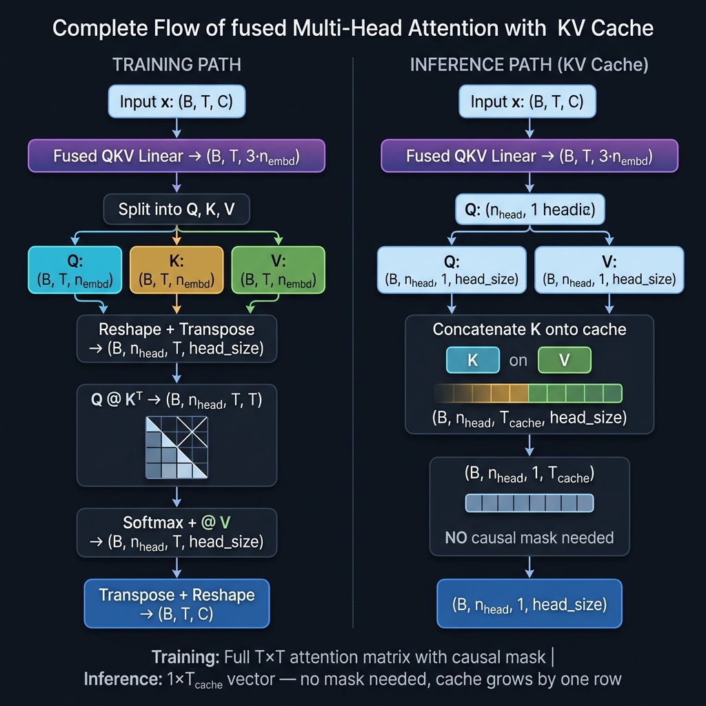
The two attention paths
There are two completely different paths depending on whether we’re training or doing inference with a KV cache.
    if not self.training:
        if self.key_cache is not None:
            self.key_cache   = torch.cat([self.key_cache, k], dim=2)   # dim=2 is T now
            self.value_cache = torch.cat([self.value_cache, v], dim=2)
        else:
            self.key_cache, self.value_cache = k, v

        scale = self.head_size ** -0.5
        attn = (q @ self.key_cache.transpose(-2, -1)) * scale  # (B, n_head, T_q, T_cache)
        attn = F.softmax(attn, dim=-1)
        out  = attn @ self.value_cache  # (B, n_head, T_q, head_size)
    else:
        scale = self.head_size ** -0.5
        attn = (q @ k.transpose(-2, -1)) * scale  # (B, n_head, T, T)
        attn = attn.masked_fill(self.tril[:T, :T] == 0, float('-inf'))  # ← missing
        attn = F.softmax(attn, dim=-1)
        out  = attn @ v

    out = out.transpose(1, 2).contiguous().view(B, T, C)  # (B, T, n_embd)
    out = self.attn_proj(out)
    return out
Training path
During training, we process the full sequence at once. The shapes trace through as:
q: (B, 4, T, 8)   k: (B, 4, T, 8)   v: (B, 4, T, 8)

q @ k.T:  (B, 4, T, 8) @ (B, 4, 8, T) → (B, 4, T, T)    ← full attention matrix
masked_fill:  upper triangle → -inf
softmax:  each row sums to 1
attn @ v: (B, 4, T, T) @ (B, 4, T, 8) → (B, 4, T, 8)    ← attended values
The causal mask (self.tril[:T, :T]) prevents each token from attending to future positions - token 3 can see tokens 0, 1, 2, 3 but not 4, 5, etc. We masked_fill with -inf so that after softmax, those positions get zero weight. This is the same mask from the original NanoGPT, just applied to (B, n_head, T, T) instead of (B, T, T) - the extra n_head dimension broadcasts.
I initially forgot this mask entirely. The model still trained and the loss decreased, but the generated text was incoherent, because during training the model could see the answer it was trying to predict. The loss was low because it was cheating, not because it was learning.
Inference path (KV cache)
During inference, T_q = 1 - we’re generating one token at a time. The fresh k and v (both (B, n_head, 1, head_size)) get concatenated onto the cache along dim=2 (the sequence dimension):
Decode step 5:
  k_new:      (B, 4, 1, 8)
  key_cache:  (B, 4, 5, 8)  ← 5 tokens already cached
  after cat:  (B, 4, 6, 8)  ← 6 tokens now

  q @ key_cache.T:  (B, 4, 1, 8) @ (B, 4, 8, 6) → (B, 4, 1, 6)   ← one row of weights
  attn @ value_cache: (B, 4, 1, 6) @ (B, 4, 6, 8) → (B, 4, 1, 8) ← attended output
Notice: no causal mask. During decode, the query is a single token attending over its entire past - there are no future tokens to mask out. The cache only contains positions 0 through T_cache-1, all of which the current token is allowed to see. This is a subtlety that confused me at first - I was applying the mask to the decode path and getting wrong shapes (the mask is (T, T) but the attention matrix is (1, T_cache), they don’t align).
Also notice dim=2 for the concatenation, not dim=-2. After the .transpose(1, 2), our shape is (B, n_head, T, head_size) - the sequence dimension is at position 2, not position 1. Getting this wrong is one of those bugs that produces a valid tensor (the cat succeeds on a different dimension) but completely wrong attention scores.
Reshaping back
After both paths, out has shape (B, n_head, T_q, head_size). We need to undo the reshape to get back to (B, T, n_embd):
out = out.transpose(1, 2).contiguous().view(B, T, C) # (B, T, n_embd)
.transpose(1, 2) swaps n_head and T back: (B, T, n_head, head_size). Then .view(B, T, C) flattens the last two dimensions back into n_embd. The .contiguous() call is necessary because .transpose() changes strides, not memory layout, and .view() requires contiguous memory. Without it, PyTorch throws a runtime error.
Then self.attn_proj(out) applies the output projection, mapping from n_embd → n_embd. This is analogous to what MultiHeadAttention.proj did after concatenating all heads in the old architecture.
Wiring it into the model
The Block class is the only place that needs to change - one line:
class Block(nn.Module):
    """ Transformer block: communication followed by computation """

    def __init__(self, n_embd, n_head):
        super().__init__()
        head_size = n_embd // n_head
        self.sa = CausalSelfAttention(n_head, head_size)  # ← was MultiHeadAttention
        self.ffwd = FeedFoward(n_embd)
        self.ln1 = nn.LayerNorm(n_embd)
        self.ln2 = nn.LayerNorm(n_embd)
The clear_kv_cache function also needs updating - it was walking Head instances that no longer exist:
def clear_kv_cache(model):
    for module in model.modules():
        if isinstance(module, CausalSelfAttention):  # ← was Head
            module.key_cache = None
            module.value_cache = None
Once these changes are in, the Head and MultiHeadAttention classes are dead code. Delete them.
Verifying equivalence
To verify, I wrote a test that initializes both architectures with the same seed, manually converts the per-head weights into the fused layout, and asserts torch.allclose on the outputs.
The weight conversion is the tricky part. The old architecture has separate Head.query.weight, Head.key.weight, Head.value.weight tensors, each (head_size, n_embd) = (8, 32). The fused qkv.weight is (96, 32). The mapping:
qkv.weight rows 0–31:   Q weights = cat([head0.query, head1.query, head2.query, head3.query])
qkv.weight rows 32–63:  K weights = cat([head0.key,   head1.key,   head2.key,   head3.key])
qkv.weight rows 64–95:  V weights = cat([head0.value, head1.value, head2.value, head3.value])
This works because qkv.split(n_embd, dim=2) reads the first n_embd=32 output dimensions as Q, the next 32 as K, the last 32 as V. And within each group, the heads are packed sequentially, which is exactly what .view(B, T, n_head, head_size) expects.
The test passes with a max absolute difference of 1.79e-07 - well within float32 precision. The fused architecture is numerically equivalent to the per-head architecture.
F.scaled_dot_product_attention
The training path has one more optimization available. Our manual attention code materializes the full (B, n_head, T, T) attention matrix in memory:
attn = (q @ k.transpose(-2, -1)) * scale   # O(T²) memory
attn = attn.masked_fill(...)
attn = F.softmax(attn, dim=-1)
out  = attn @ v
This is three separate operations, three kernel launches, and O(T²) memory for the attention matrix. PyTorch 2.0’s F.scaled_dot_product_attention replaces all of it with a single fused kernel that, on CUDA, dispatches to FlashAttention - an algorithm that computes attention in tiles that fit in GPU SRAM, never materializing the full attention matrix:
# Training branch - one line replaces four:
out = F.scaled_dot_product_attention(q, k, v, is_causal=True)
| Manual attention | F.scaled_dot_product_attention |
|
|---|---|---|
| Memory | O(T²) - full attention matrix | O(T) - tiled in SRAM |
| Kernel launches | 3 separate ops | 1 fused kernel |
| Causal mask | Manual masked_fill |
is_causal=True handles it |
| Speed on GPU | baseline | ~2–4× faster for long sequences |
For the inference path, the same function works but with is_causal=False - because during decode, T_q=1 and T_k=T_cache have different lengths, and the single-token query should attend freely to all cached positions:
# Inference branch:
out = F.scaled_dot_product_attention(
    q, self.key_cache, self.value_cache, is_causal=False
)
At our scale (T=64, CPU), the speedup is negligible. On GPU with T=512+, it’s dramatic. This is why every production model uses F.scaled_dot_product_attention or its Triton equivalents: the memory savings alone make long-context attention feasible.
Shape walkthrough: one full cycle
Let me trace the complete shapes through a prefill + one decode step, using our actual hyperparameters: B=1, T=9 (prompt), n_embd=32, n_head=4, head_size=8.
Prefill (9-token prompt):
model.forward(idx)  # idx: (1, 9)
  tok_emb: (1, 9, 32)    # token embedding lookup
  pos_emb: (9, 32)        # position embedding for positions 0..8
  x:       (1, 9, 32)     # tok_emb + pos_emb (broadcast)

  → CausalSelfAttention.forward(x):
    qkv = self.qkv(x):    (1, 9, 96)   # one fused projection
    q, k, v = split:      each (1, 9, 32)

    q = view + transpose:  (1, 4, 9, 8)  # 4 heads, 9 positions, 8 dims
    k = view + transpose:  (1, 4, 9, 8)
    v = view + transpose:  (1, 4, 9, 8)

    key_cache is None → set directly
    key_cache:   (1, 4, 9, 8)
    value_cache: (1, 4, 9, 8)

    attn = q @ key_cache.T: (1,4,9,8) @ (1,4,8,9) → (1, 4, 9, 9)
    out  = attn @ value_cache:  (1,4,9,9) @ (1,4,9,8) → (1, 4, 9, 8)

    out = transpose + view: (1, 9, 32)
    out = attn_proj(out):   (1, 9, 32)
Decode step 0 (one new token):
model.forward(idx_next, start_pos=9)  # idx_next: (1, 1)
  tok_emb: (1, 1, 32)
  pos_emb: (1, 32)       # position embedding for position 9
  x:       (1, 1, 32)

  → CausalSelfAttention.forward(x):
    qkv = self.qkv(x):    (1, 1, 96)
    q, k, v = split:      each (1, 1, 32)

    q = view + transpose:  (1, 4, 1, 8)
    k = view + transpose:  (1, 4, 1, 8)
    v = view + transpose:  (1, 4, 1, 8)

    key_cache: cat[(1,4,9,8), (1,4,1,8)] → (1, 4, 10, 8)   ← grew by 1
    value_cache: cat[(1,4,9,8), (1,4,1,8)] → (1, 4, 10, 8)

    attn = q @ key_cache.T: (1,4,1,8) @ (1,4,8,10) → (1, 4, 1, 10)
    out  = attn @ value_cache: (1,4,1,10) @ (1,4,10,8) → (1, 4, 1, 8)

    out = transpose + view: (1, 1, 32)
    out = attn_proj(out):   (1, 1, 32)
Compare this to the old per-head architecture from the KV cache post: there, each head had its own (1, T, 16) tensors and ran its own attention. Here, all 4 heads are packed into a single (1, 4, T, 8) tensor and run as one batched matmul. The computation is identical. The dispatch is not.
Things that went wrong
Forgot super().__init__(). Without calling the parent nn.Module.__init__(), PyTorch doesn’t set up the internal parameter tracking machinery. The class instantiates fine, but model.parameters() returns nothing - so the optimizer has zero parameters to update. The model appears to train (no errors), but the loss doesn’t decrease. This is a classic PyTorch gotcha.
Forgot the causal mask in training. The model trained and the loss dropped quickly - too quickly. Without the mask, each token could see its target during training, so the model was memorizing rather than learning to predict. The generated text was gibberish despite a low training loss. Adding attn.masked_fill(self.tril[:T, :T] == 0, float('-inf')) fixed it immediately.
Cache concatenation on wrong dimension. After .transpose(1, 2), the shape is (B, n_head, T, head_size) - the sequence dimension is at index 2. I initially wrote torch.cat([self.key_cache, k], dim=-2) which happened to work since dim=-2 is also dim=2 for a 4D tensor. But when I changed it to dim=1 (thinking “sequence is the second dimension”), the cache grew along the head dimension instead. Each “head” ended up with a mix of keys from different heads, and the attention scores were garbage. Always be explicit about which dimension you’re concatenating on.
Missing .contiguous() before .view(). The transpose creates a non-contiguous tensor, and .view() requires contiguous memory. PyTorch throws RuntimeError: view size is not compatible with input tensor's size and stride. The fix is .contiguous() between the transpose and the view, or use .reshape() which handles this internally (but may copy data).
You can see the complete code on GitHub: https://github.com/czhou578/nanoGPT-inference/blob/fused-att/nanogpt-fused-attention.py
CZ