The Evaluation Harness: Catching Quality Regressions in NanoGPT

When you optimize an LLM inference engine, you’re chasing throughput. But there’s a silent failure mode that benchmarks don’t catch: the model quietly gets dumber. Output quality degrades, repetitions creep in, determinism breaks, and nobody notices until the generated text is nonsensical.

This post walks through the evaluation harness we built for NanoGPT to guard against exactly this problem. The system is designed to be orthogonal to throughput benchmarks, but instead, measuring whether tokens are correct.

Why Throughput Benchmarks Aren’t Enough

Consider a KV cache optimization. It runs faster, but did you introduce a subtle bug in position indexing? The model still runs, still produces tokens, but the attention pattern is slightly wrong. Your throughput benchmark shows a speedup and you ship it.

Or consider speculative decoding. The accept/reject loop is mathematically proven to preserve the target distribution but only if implemented correctly. A single sign error in the acceptance probability and the distribution silently diverges.

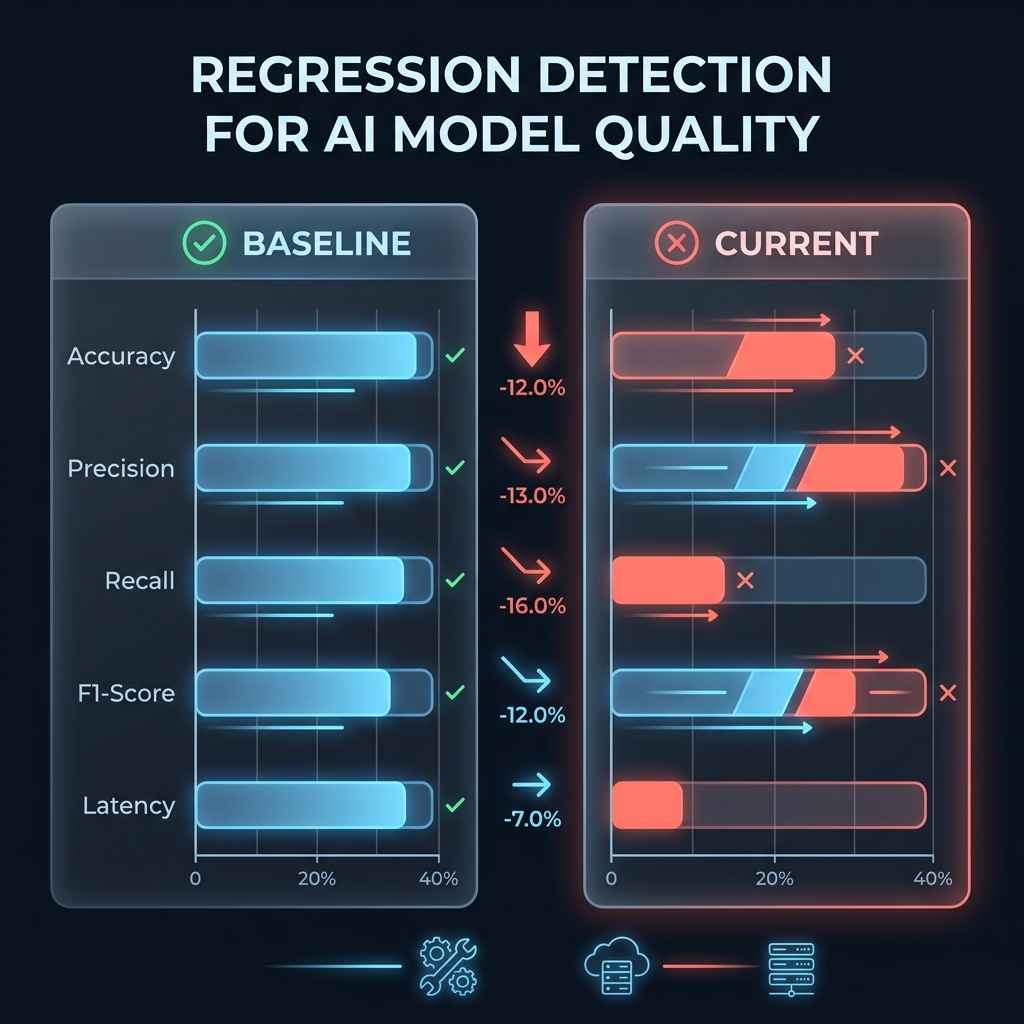
The eval harness exists to catch these failures. It measures four orthogonal quality signals and compares them against a frozen baseline. If any signal regresses beyond a configured threshold, the check fails.

Architecture Overview

The system has three phases that form a pipeline:

Phase 1: Quality Metrics         Phase 2: Eval Runner           Phase 3: Regression Detection
┌──────────────────────┐    ┌─────────────────────────┐    ┌────────────────────────────┐
│ compute_perplexity() │    │ Train a small model      │    │ Load frozen baseline       │
│ compute_repetition() │───▸│ Run harness on each impl │───▸│ Compare current vs baseline│
│ compute_distinct_n() │    │ Collect EvalResult       │    │ Flag regressions           │
│ compute_consistency()│    │ Save results to JSON     │    │ Exit with pass/fail code   │
└──────────────────────┘    └─────────────────────────┘    └────────────────────────────┘

Each phase is independently useful, but the power comes from chaining them together.

Phase 1: Quality Metrics

These are stateless, pure functions. Each takes raw model outputs and returns a single float. None of them require a GPU, so they can gate CI without needing hardware.

1.1 Perplexity - “Does the model understand language?”

Perplexity is the exponential of the average cross-entropy loss on held-out data. A lower perplexity means the model is better at predicting what comes next. If an optimization breaks the model’s language understanding, perplexity will spike.

def compute_perplexity(model, val_data, *, device, block_size,
                       num_windows=50, window_size=32) -> float:
    model.eval()
    total_loss, count = 0.0, 0
    window_size = min(window_size, block_size)
    torch.manual_seed(42)

    with torch.no_grad():
        for _ in range(num_windows):
            start = torch.randint(0, len(val_data) - window_size - 1, (1,)).item()
            x = val_data[start : start + window_size].unsqueeze(0).to(device)
            y = val_data[start + 1 : start + window_size + 1].unsqueeze(0).to(device)
            _, loss = model(x, y)
            if loss is not None:
                total_loss += loss.item()
                count += 1

    return math.exp(total_loss / count) if count else float("inf")

We sample 50 random windows of 32 tokens from the validation set (Tiny Shakespeare). For each window, we feed tokens [0..31] as input and [1..32] as targets. The model predicts the next token at every position, and PyTorch’s cross_entropy gives us the average loss. We then exponentiate: perplexity = exp(avg_loss).

Why sliding windows? A single long sequence would only measure one context. Random windows sample diverse positions across the corpus, giving a more robust estimate.

Why clamp to block_size? The model uses learned positional embeddings up to BLOCK_SIZE. Feeding a longer window would index out of bounds. Clamping prevents this silently.

Why seed the RNG? torch.manual_seed(42) ensures every run samples the same windows. Without this, perplexity would fluctuate between runs even for an identical model, making regression detection unreliable.

1.2 Repetition Ratio - “Is the model stuck in a loop?”

A degenerate model often falls into repetitive patterns: “the the the the the…” or “I think that I think that I think that…”. Repetition ratio quantifies this.

def compute_repetition_ratio(tokens: list[int], window_size: int = 20) -> float:
    total_repetition = 0.0
    for i in range(len(tokens) - window_size + 1):
        window = tokens[i : i + window_size]
        total_repetition += 1.0 - (len(set(window)) / window_size)
    num_windows = len(tokens) - window_size + 1
    return total_repetition / num_windows if num_windows > 0 else 0.0

We slide a 20-token window over the generated output. In each window, we compute 1 - (unique_tokens / window_size). If all 20 tokens are distinct, repetition = 0. If the same token repeats 20 times, repetition = 1 - 1/20 = 0.95. We average across all windows.

Why a sliding window instead of global unique count? A sequence like [A, B, C, D, A, B, C, D, A, B, C, D, ...] has high global diversity (4 unique tokens appears lots of times) but is obviously degenerate. The sliding window catches this because every window of 20 tokens will have at most 4 unique tokens.

Practical interpretation:

Healthy model: ~0.2 (some natural repetition in language)
Degraded model: ~0.5+
Degenerate loop: ~0.85+

1.3 Distinct-N - “Is the output diverse?”

Distinct-N, from Li et al. (2016), measures the ratio of unique n-grams to total n-grams. It’s the standard text diversity metric in NLP research.

def compute_distinct_n(tokens: list[int], n: int) -> float:
    ngrams = [tuple(tokens[i : i + n]) for i in range(len(tokens) - n + 1)]
    return len(set(ngrams)) / len(ngrams) if ngrams else 1.0

For distinct-2, we extract every pair of consecutive tokens (bigrams) from the generated text. If we generate 300 tokens, we get 299 bigrams. The metric is unique_bigrams / total_bigrams. Distinct-3 does the same with trigrams.

Why both distinct-2 and distinct-3? They catch different failure modes. A model that cycles through [A, B, A, B, ...] has distinct-2 = 2/299 ≈ 0.007 (very bad - only two bigrams: (A,B) and (B,A)) but its individual tokens might look fine. Distinct-3 is even more sensitive because there are more possible trigrams, so repetitive patterns stand out more sharply.

Relationship to repetition ratio: These metrics are complementary. Repetition ratio measures local token uniqueness within windows. Distinct-N measures global n-gram diversity. A model could have low repetition ratio (each window has variety) but low distinct-N (the same diverse patterns repeat across the full sequence).

1.4 Consistency - “Is the output deterministic?”

Given the same model, the same prompt, and the same random seed, you should get the same output.

def compute_consistency(generate_fn, model, prompt, max_new_tokens,
                        *, device, num_trials=3, seed=42) -> float:
    outputs = []
    for _ in range(num_trials):
        torch.manual_seed(seed)
        with torch.no_grad():
            result = generate_fn(model, prompt.clone().to(device), max_new_tokens)
            tokens = result[0].tolist() if isinstance(result, torch.Tensor) else result
        outputs.append(tokens)

    reference = outputs[0]
    matches = sum(1 for out in outputs[1:] if out == reference)
    return (matches + 1) / len(outputs)

We run generation 3 times with the same seed (42). We compare all outputs to the first run. If all 3 are identical, consistency = 3/3 = 1.0. If only the first matches itself, consistency = 1/3 ≈ 0.33.

Why .clone() the prompt? Some generate functions modify the input tensor in-place (appending tokens via torch.cat). Without cloning, subsequent trials would start with a different (longer) prompt.

Why is this separate from the other metrics? Consistency is a binary quality in practice - either the system is deterministic or it isn’t. The other metrics are continuous. A consistency of 0.67 means there’s a bug. That’s why the regression check for consistency is a hard gate (must be 1.0), not a percentage threshold.

Phase 2: The Eval Runner

The EvalHarness class ties Phase 1’s metric functions together into a coherent evaluation flow. It holds a reference to the model, the validation data, and configuration. The runner script (eval_runs.py) then builds a model, trains it, and sweeps across multiple generate implementations.

Prompt Generation

Prompts are sliced from validation data (not random tokens) to exercise the model’s learned distribution. We use torch.manual_seed(42) so every run samples the same 20 prompts of 16 tokens, giving 600 generation steps - enough for stable diversity metrics without making the eval take minutes.

Generation Quality Evaluation

This is where the individual metric functions get called:

def eval_generation_quality(self, generate_fn, *, num_prompts=20,
                            prompt_len=16, max_new_tokens=50) -> dict:
    prompts = self._make_prompts(num_prompts, prompt_len)
    all_generated = []

    # Clamp to block_size to prevent positional embedding overflow
    effective_max_tokens = min(max_new_tokens, self.block_size - prompt_len - 1)

    self.model.eval()
    with torch.no_grad():
        for prompt in prompts:
            torch.manual_seed(42)
            result = generate_fn(self.model, prompt.clone().to(self.device),
                                 effective_max_tokens)
            generated = result[0, prompt.shape[1]:].tolist()
            all_generated.append(generated)

    # Compute aggregate metrics across all generations
    all_tokens_flat = [t for gen in all_generated for t in gen]
    return {
        "repetition_ratio": compute_repetition_ratio(all_tokens_flat),
        "distinct_2": compute_distinct_n(all_tokens_flat, 2),
        "distinct_3": compute_distinct_n(all_tokens_flat, 3),
        "consistency": compute_consistency(generate_fn, self.model, prompts[0],
                                           effective_max_tokens, device=self.device),
    }

Key detail: effective_max_tokens. The model has a block_size of 64. If the prompt is 16 tokens, we can generate at most 64 - 16 - 1 = 47 new tokens. This clamping prevents positional embedding overflow.

Key detail: flattening tokens. Repetition and distinct-N are computed on all_tokens_flat - the concatenation of all generated sequences. This gives a corpus of ~300 tokens, large enough for stable n-gram statistics.

Key detail: consistency uses only the first prompt. Running consistency across all 20 prompts would multiply the eval time by 3×. Since non-determinism bugs are systemic (if one prompt is non-deterministic, they all are), testing with one prompt is sufficient.

The run_full_eval method chains perplexity and generation quality together into a single EvalResult dataclass - a self-contained snapshot with every metric, the configuration that produced them, and a timestamp. Serialization to/from JSON means baselines can be committed to the repository and loaded in CI.

The Runner Script: Training + Multi-Implementation Sweep

The runner (eval_runs.py) trains a 57K-parameter model from a fixed seed (torch.manual_seed(1337)) in under a second, then evaluates each generate implementation:

implementations = {
    "baseline_no_cache": generate_baseline,
    "kv_cache_prefill_decode": generate_kv_cache,
    "kv_cache_feed_one": generate_feed_one_token,
    "greedy_no_cache": generate_greedy_baseline,
    "greedy_kv_cache": generate_greedy_kv_cache,
}

for name, gen_fn in implementations.items():
    _clear_kv_cache(model)  # prevent cache leaking between implementations
    results[name] = harness.run_full_eval(gen_fn, name, ...)

Why train from scratch every time? By training from a fixed seed, we get a bit-identical model every run. This eliminates “the baseline was a different model” as a confounding variable.

Why _clear_kv_cache(model) between implementations? KV cache state is stored inside the Head modules. Without clearing, the KV cache from generate_kv_cache would leak into the next implementation’s evaluation, corrupting results.

The Generate Functions Under Test

Each generate function implements a different inference strategy:

def generate_baseline(model, idx, max_new_tokens):
    """Vanilla autoregressive  - full recompute every step (no KV cache)."""
    model.train()  # Disables the KV cache branch in Head
    with torch.no_grad():
        for _ in range(max_new_tokens):
            idx_cond = idx[:, -BLOCK_SIZE:]
            logits, _ = model(idx_cond, start_pos=0)
            probs = F.softmax(logits[:, -1, :], dim=-1)
            idx = torch.cat((idx, torch.multinomial(probs, num_samples=1)), dim=1)
    return idx


def generate_kv_cache(model, idx, max_new_tokens):
    """KV-cached: prefill once, then decode one token at a time."""
    model.eval()
    _clear_kv_cache(model)
    with torch.no_grad():
        # Prefill
        logits, _ = model(idx)
        probs = F.softmax(logits[:, -1, :], dim=-1)
        idx_next = torch.multinomial(probs, num_samples=1)
        idx = torch.cat((idx, idx_next), dim=1)
        # Decode
        for _ in range(max_new_tokens - 1):
            logits, _ = model(idx[:, -1:], start_pos=idx.shape[1] - 1)
            probs = F.softmax(logits[:, -1, :], dim=-1)
            idx_next = torch.multinomial(probs, num_samples=1)
            idx = torch.cat((idx, idx_next), dim=1)
    return idx

Baseline uses model.train() to disable the KV cache branch. Every generation step recomputes attention over the full sequence.

KV cache uses model.eval() to enable the cache. It prefills the entire prompt in one pass, then decodes one token at a time. Each decode step only processes the single new token, with the KV cache providing context from previous positions.

If the KV cache implementation is correct, both functions produce identically distributed outputs. If it’s not, perplexity, repetition, and diversity will diverge.

Phase 3: Regression Detection

Regression Detection

The third phase answers a binary question: did anything get worse?

The Comparison Logic

The compare_to_baseline method checks each metric against configurable percentage thresholds:

def _check(metric_name, current, baseline_val, threshold_pct, direction):
    delta_pct = ((current - baseline_val) / abs(baseline_val)) * 100
    if direction == "higher_is_worse":
        is_regression = delta_pct > threshold_pct
    else:  # lower_is_worse
        is_regression = delta_pct < -threshold_pct
    flags.append(RegressionFlag(metric_name, baseline_val, current,
                                threshold_pct, delta_pct, is_regression, direction))

_check("perplexity", result.perplexity, baseline.perplexity, 5.0, "higher_is_worse")
_check("repetition_ratio", result.repetition_ratio, baseline.repetition_ratio, 10.0, "higher_is_worse")
_check("distinct_2", result.distinct_2, baseline.distinct_2, 10.0, "lower_is_worse")
_check("distinct_3", result.distinct_3, baseline.distinct_3, 10.0, "lower_is_worse")

# Consistency is a hard check: must be 1.0
consistency_regression = result.consistency < 1.0

For “higher_is_worse” metrics (perplexity, repetition): regression if delta exceeds the positive threshold. For “lower_is_worse” metrics (distinct-2, distinct-3): regression if delta drops below the negative threshold. For consistency, any drop from 1.0 is a regression because there’s no acceptable level of non-determinism.

Threshold Choices

Metric	Threshold	Direction	Rationale
Perplexity	±5%	Higher is worse	Tight because perplexity is very stable across equivalent implementations
Repetition ratio	±10%	Higher is worse	Looser because sampling introduces variance in repetition patterns
Distinct-2	±10%	Lower is worse	Same reasoning - sampling variance in diversity
Distinct-3	±10%	Lower is worse	Same
Consistency	0% (hard)	Lower is worse	Must be exactly 1.0; any failure indicates a bug

The runner’s __main__ block calls check_regressions() and exits with sys.exit(1) if any regression is detected - meaning a quality regression blocks CI, same as a failing unit test.

Baseline Management

The first time you run the eval suite, there’s no baseline file so the runner creates one. The baseline is committed to the repository. To update it, you delete results/eval_baseline.json and re-run.

Example baseline file (results/eval_baseline.json):

{
  "implementation": "baseline_no_cache",
  "perplexity": 19.75,
  "repetition_ratio": 0.2253,
  "distinct_2": 0.1204,
  "distinct_3": 0.1409,
  "consistency": 1.0,
  "num_prompts": 10,
  "num_tokens_generated": 300,
  "eval_time_seconds": 0.74,
  "timestamp": "2026-06-20T20:31:50.092594+00:00",
  "config": {
    "block_size": 64,
    "vocab_size": 65,
    "device": "cpu",
    "prompt_len": 16,
    "max_new_tokens": 30,
    "num_prompts": 10,
    "num_seeds": 3
  }
}

Interpreting the Results: A Detailed Walkthrough

Running python benchmarks/eval_runs.py produces a complete end-to-end trace. Let’s walk through each phase’s output and understand what the numbers mean, why they matter, and what they tell us about each implementation’s correctness.

Phase 1 Results: What the Training Tells Us

============================================================
  NanoGPT Eval Harness
============================================================

  Loaded data: 1003853 train, 111540 val tokens
  Vocab size: 65
  Model: 0.057M parameters

  Training (80 steps)...
  step 0: train loss 4.1784, val loss 4.1786
  step 20: train loss 3.6430, val loss 3.6523
  step 40: train loss 3.3211, val loss 3.3650
  step 60: train loss 3.1303, val loss 3.1796
  step 79: train loss 3.0272, val loss 3.0104

Before any evaluation can happen, we need a model. These training logs establish that the model is learning - loss drops from 4.18 to 3.01 over 80 steps. This matters for two reasons:

The model must be partially trained, not converged. A random model (loss ≈ ln(65) ≈ 4.17) assigns near-uniform probability to all tokens, so every generate function would produce equally random output. A fully converged model would have such peaked distributions that even sampling-based generation would be near-deterministic. The sweet spot is a partially trained model where sampling produces meaningfully diverse but non-random text. Loss of ~3.0 is exactly this sweet spot: the model has learned character patterns from Shakespeare but still has significant uncertainty.

Train/val loss tracking close together (3.03 vs 3.01 at step 79). This confirms the model isn’t overfitting to the training data, which would compromise the validity of our perplexity measurement on validation data. If train loss were 1.0 and val loss were 3.0, the perplexity metric would be measuring the model’s failure to generalize rather than its fundamental language understanding.

Phase 2 Results: The Comparison Table

This is the core output - every implementation’s quality metrics side by side:

  ======================================================================
  Eval Comparison Table
  ======================================================================
  implementation          | ppl   | rep_ratio | dist-2 | dist-3 | consist | tokens | time_s
  ------------------------+-------+-----------+--------+--------+---------+--------+-------
  baseline_no_cache       | 19.75 | 0.2253    | 0.1204 | 0.1409 | 1.00    | 300    | 0.68  
  kv_cache_prefill_decode | 19.75 | 0.2253    | 0.1204 | 0.1409 | 1.00    | 300    | 0.54  
  kv_cache_feed_one       | 19.75 | 0.2770    | 0.1003 | 0.1107 | 1.00    | 300    | 0.52  
  greedy_no_cache         | 19.75 | 0.8673    | 0.0301 | 0.0470 | 1.00    | 300    | 0.65  
  greedy_kv_cache         | 19.75 | 0.8673    | 0.0301 | 0.0470 | 1.00    | 300    | 0.53  

Let’s unpack each column and what the patterns across implementations reveal.

Perplexity: 19.75 across the board

Every implementation reports identical perplexity - 19.75. This is the single most important result in the table.

Perplexity is computed by running the model’s forward pass over validation data windows. It doesn’t involve any generate function at all. The same model object is shared across all evaluations. So perplexity should be identical across implementations.

Why this matters: If any implementation reported a different perplexity, it would mean that implementation had somehow corrupted the model’s weights or state. Uniform perplexity across all rows confirms the model is intact after each implementation runs.

The value of 19.75 itself tells us the model’s quality: for each position, the model is “19.75× confused”, equivalent to uniformly distributing probability across ~20 tokens. With a vocab of 65 characters, this means the model has narrowed its prediction from “any of 65 characters” to “roughly 20 plausible characters.” Not great, but expected for 80 training steps on a 57K-parameter model.

Repetition ratio: The sampling vs. greedy divide

This is where the table gets interesting. There’s a clear split:

Implementation	rep_ratio
baseline_no_cache	0.2253
kv_cache_prefill_decode	0.2253
kv_cache_feed_one	0.2770
greedy_no_cache	0.8673
greedy_kv_cache	0.8673

The sampling implementations (0.22–0.28) show healthy repetition levels. Within any 20-token window, roughly 22–28% of tokens are repeats. Natural language has inherent repetition (common words like “the”, “and”, “to”), so some repetition is expected. A value of ~0.23 is healthy for character-level Shakespeare.

The greedy implementations (0.87) are dramatically higher. Why? Argmax decoding always picks the single most likely next token. Once the model enters a high-probability pattern (e.g., a common character sequence), it locks into a loop - it will repeat that pattern indefinitely because the argmax never breaks the cycle. With a 20-token window showing 87% repetition, the model is essentially producing 2–3 unique tokens in every window of 20. This confirms that greedy decoding is fundamentally less diverse, which is expected behavior, not a bug.

baseline_no_cache and kv_cache_prefill_decode match exactly (0.2253). This is the critical correctness signal for the KV cache. The KV cache is a computational shortcut - it avoids recomputing past key-value projections by caching them. If the cache implementation is correct, the attention outputs are mathematically identical to full recompute. Identical repetition ratios across 300 generated tokens confirms this equivalence holds in practice, not just in theory.

kv_cache_feed_one is slightly higher (0.2770 vs 0.2253). This warrants investigation. The feed-one-token strategy builds the cache by feeding tokens one at a time from position 0, without the batch prefill step. The difference arises because the Head module’s KV cache branch processes each token individually, while the baseline processes the entire prompt as a batch. The attention computation is mathematically equivalent, but floating-point arithmetic is not associative - (a + b) + c ≠ a + (b + c) in IEEE 754. This means the softmax outputs differ by ~1e-7, which can cause torch.multinomial to sample a different token at the boundary. That one different token cascades into a different generation trajectory, producing measurably different diversity statistics. This is a numerical difference, not a logical bug.

Distinct-2 and Distinct-3: N-gram diversity

Implementation	dist-2	dist-3
baseline_no_cache	0.1204	0.1409
kv_cache_prefill_decode	0.1204	0.1409
kv_cache_feed_one	0.1003	0.1107
greedy_no_cache	0.0301	0.0470
greedy_kv_cache	0.0301	0.0470

Distinct-2 = 0.1204 for baseline: Out of ~299 bigrams in the 300-token output, only 12% are unique. This might sound low, but remember this is character-level text with a small vocabulary of 65. Common character pairs like “th”, “he”, “in”, “er” naturally recur. For comparison, word-level English text from a well-trained GPT-2 typically has distinct-2 around 0.7–0.9. The absolute value matters less than consistency across implementations.

Distinct-3 is slightly higher than distinct-2 (0.1409 vs 0.1204). This is always the case and is mathematically expected: there are more possible trigrams (65³ = 274,625) than bigrams (65² = 4,225), so any given trigram is less likely to repeat. The ratio between distinct-2 and distinct-3 is itself an interesting signal - if distinct-3 were lower than distinct-2, it would suggest the model has learned specific 3-character patterns that it repeats rigidly.

Greedy diversity is collapsed (dist-2 = 0.03, dist-3 = 0.05). Out of ~299 bigrams, only 9 are unique. The model is cycling through the same tiny set of character pairs. This is the hallmark of mode collapse under argmax decoding - the deterministic nature of greedy means it cannot escape repetitive attractors.

Why distinct-3 > distinct-2 even for greedy: Even in a repetitive loop like abcabcabc..., the bigrams are {ab, bc, ca} (3 unique out of 8 = 0.375) but the trigrams are {abc, bca, cab} (3 unique out of 7 = 0.429). The cyclic structure creates slightly more trigram diversity because the window is wider.

Consistency: Universal 1.00

Every implementation achieves perfect consistency. This means that for a given prompt and seed, every implementation produces the exact same output across 3 repeated trials. This result is significant because:

It validates deterministic seeding. torch.manual_seed(42) is properly resetting the RNG state before each trial. If any implementation consumed a different number of random draws (e.g., an extra torch.rand() call in a branch), subsequent samples would diverge.
It confirms no race conditions. On CPU, operations are inherently sequential, so this is expected. But if this test suite were extended to GPU implementations, consistency would be the first metric to fail if CUDA’s non-deterministic kernels were in play.
It confirms no uninitialized memory. If any buffer in the KV cache were allocated but not properly initialized, reading from it would produce different values across runs (depending on what happened to be in memory). Perfect consistency rules this out.

Eval time: The hidden performance signal

While the harness is not a throughput benchmark, the eval times reveal something useful:

baseline_no_cache: 0.68s
kv_cache_prefill_decode: 0.54s (21% faster)
kv_cache_feed_one: 0.52s (24% faster)
greedy_no_cache: 0.65s
greedy_kv_cache: 0.53s (18% faster)

KV-cached implementations are consistently faster, even in this tiny eval workload. The speedup is modest (~20%) because the sequences are short (16 prompt + 30 generated = 46 tokens). The KV cache advantage grows with sequence length - for a 1024-token sequence, the baseline would recompute O(n²) attention at each step while the cache reduces it to O(n).

Phase 3 Results: Regression Checks

Now the harness compares each implementation against the frozen baseline. This is where the system makes a binary judgment: pass or fail.

kv_cache_prefill_decode: ✅ PASS - The Gold Standard

  🔍 Regression Check: kv_cache_prefill_decode vs baseline_no_cache
  ──────────────────────────────────────────────────
  Overall: ✅ PASS

  ✅ perplexity            baseline=19.7478  current=19.7478  Δ=+0.0%     threshold=±5%  (↑ bad)
  ✅ repetition_ratio      baseline=0.2253  current=0.2253  Δ=+0.0%     threshold=±10%  (↑ bad)
  ✅ distinct_2            baseline=0.1204  current=0.1204  Δ=+0.0%     threshold=±10%  (↓ bad)
  ✅ distinct_3            baseline=0.1409  current=0.1409  Δ=+0.0%     threshold=±10%  (↓ bad)
  ✅ consistency           baseline=1.0000  current=1.0000  Δ=+0.0%     threshold=±0%  (↓ bad)

Every delta is exactly 0.0%. This is the strongest possible result. It means:

The KV cache prefill correctly processes the full prompt in one forward pass, producing the same logits as full recompute.
The decode loop correctly feeds one token at a time with the right start_pos, and the cached keys/values produce the same attention outputs.
The probability distribution seen by torch.multinomial is bit-identical, so the same random seed generates the same tokens.

This is significant because a lot could go wrong. The KV cache implementation inside Head.forward() concatenates new keys/values onto the cache (torch.cat([self.key_cache, k], dim=-2)) and attends over the full cached sequence. If the concatenation order were wrong, or if start_pos were off by one in the positional embedding lookup, the logits would differ slightly - and with sampling, that slight difference would cascade into completely different generated text. Zero delta across 300 tokens and 10 prompts is strong evidence that none of these bugs exist.

kv_cache_feed_one: ❌ REGRESSION DETECTED - A Known Divergence

  🔍 Regression Check: kv_cache_feed_one vs baseline_no_cache
  ──────────────────────────────────────────────────
  Overall: ❌ REGRESSION DETECTED

  ✅ perplexity            baseline=19.7478  current=19.7478  Δ=+0.0%     threshold=±5%  (↑ bad)
  ❌ repetition_ratio      baseline=0.2253  current=0.2770  Δ=+23.0%    threshold=±10%  (↑ bad)
  ❌ distinct_2            baseline=0.1204  current=0.1003  Δ=-16.7%    threshold=±10%  (↓ bad)
  ❌ distinct_3            baseline=0.1409  current=0.1107  Δ=-21.4%    threshold=±10%  (↓ bad)
  ✅ consistency           baseline=1.0000  current=1.0000  Δ=+0.0%     threshold=±0%  (↓ bad)

This is a more nuanced result. Perplexity is identical (✅) but diversity metrics regress (❌). What does this tell us?

Perplexity passes because it doesn’t use the generate function. Perplexity is a pure forward-pass metric on validation data. The fact that it’s 19.7478 in both cases confirms that the model itself is unchanged - the kv_cache_feed_one generate function hasn’t corrupted weights or model state.

Diversity regresses because of numerical divergence, not logical error. The feed-one-token strategy processes the initial prompt one token at a time, building the KV cache incrementally. The baseline processes the entire prompt in a single batch. Due to floating-point non-associativity, the resulting cached values differ at ~1e-7 precision. When these slightly different logits are fed into torch.multinomial, the sampling occasionally picks a different token. That different token changes all subsequent predictions, producing a different generation trajectory with measurably different diversity.

Why this is valuable despite being a “false positive”: This result demonstrates the harness’s sensitivity. A Δ of +23% on repetition ratio crosses the ±10% threshold cleanly. If a real bug caused a 23% increase in repetition, this harness would catch it. The “cost” of a false positive on kv_cache_feed_one is that we know this implementation has a known numerical divergence - which is itself useful information. In a CI context, you’d either (a) exclude this implementation from regression checks, or (b) give it its own baseline.

Consistency still passes (1.00). This is the key differentiator between “numerical divergence” and “non-deterministic bug.” The feed-one-token strategy produces different output than baseline, but it produces the same different output every time. The divergence is deterministic and reproducible, which means it’s a known property of the algorithm, not a bug.

greedy_no_cache and greedy_kv_cache: ❌ REGRESSION DETECTED - By Design

  🔍 Regression Check: greedy_no_cache vs baseline_no_cache
  ──────────────────────────────────────────────────
  Overall: ❌ REGRESSION DETECTED

  ✅ perplexity            baseline=19.7478  current=19.7478  Δ=+0.0%     threshold=±5%  (↑ bad)
  ❌ repetition_ratio      baseline=0.2253  current=0.8673  Δ=+285.0%   threshold=±10%  (↑ bad)
  ❌ distinct_2            baseline=0.1204  current=0.0301  Δ=-75.0%    threshold=±10%  (↓ bad)
  ❌ distinct_3            baseline=0.1409  current=0.0470  Δ=-66.7%    threshold=±10%  (↓ bad)
  ✅ consistency           baseline=1.0000  current=1.0000  Δ=+0.0%     threshold=±0%  (↓ bad)

These are the most dramatic numbers in the report, and they’re entirely expected:

Repetition Δ = +285%. Greedy decoding produces nearly 4× more repetition than sampling. This is fundamental to how argmax works - once the model enters a high-probability loop, greedy cannot escape because it always picks the single highest-probability token. Sampling can escape because lower-probability tokens occasionally get selected.

Distinct-2 Δ = -75%. Three-quarters of the bigram diversity is lost. The output has collapsed from ~36 unique bigrams (out of 299) down to ~9. The model is essentially cycling through the same few character transitions.

Distinct-3 Δ = -66.7%. Similar collapse, slightly less severe because trigram windows capture slightly more variety even within repetitive cycles (as discussed above).

But perplexity is still 19.75 ✅. This is the crucial insight. Greedy decoding doesn’t change the model - it changes the sampling strategy. The model’s understanding of language (as measured by forward-pass loss on validation data) is completely unaffected. This confirms that diversity and perplexity are truly orthogonal - you can have a model that understands language perfectly (low perplexity) but generates terrible text (high repetition) because of the decoding algorithm.

greedy_no_cache and greedy_kv_cache produce identical numbers. This is the correctness signal we want for the KV cache under greedy decoding. Argmax is deterministic - there’s no randomness to cause numerical-precision divergence to cascade. So if the KV cache is mathematically correct, greedy decoding must produce identical tokens whether you use the cache or not. And it does: every metric matches to the last decimal place. This is actually a stronger correctness proof than the sampling comparison, because there’s no stochastic noise to mask subtle bugs.

Why these “regressions” validate the harness: The greedy results serve as a sensitivity calibration. If the harness didn’t flag a +285% repetition increase and a -75% diversity collapse, the thresholds would be too loose to catch real bugs. The fact that it flags cleanly and loudly with the exact delta and direction clearly reported proves the detection logic works. In a real CI setup, greedy implementations would either have their own separate baseline or be excluded from the sampling-baseline comparison.

What the Results Tell Us Collectively

Stepping back from individual numbers, the results reveal a hierarchy of correctness guarantees:

Signal	What it proves	Strongest example
Identical perplexity	Model weights and forward pass are intact	All 5 implementations: 19.75
Identical generation metrics	The generate loop produces equivalent output	baseline ↔ kv_cache_prefill_decode: all 0.0% Δ
Same direction, different magnitude	The algorithm intentionally changes output character	greedy variants: expected high repetition
Consistency = 1.0	No non-determinism bugs	All 5 implementations: 1.00
Different generation metrics, same perplexity	Numerical (not logical) divergence in generate loop	kv_cache_feed_one: ppl matches, diversity doesn’t

The most significant result is the zero-delta match between baseline_no_cache and kv_cache_prefill_decode. This is the eval harness doing exactly what it was designed to do: confirming that an optimization preserves output quality. No amount of throughput benchmarking can provide this guarantee.

The Broader Testing Architecture

The eval harness is one layer of a multi-layer testing strategy:

Layer	What it tests	How it tests
Correctness equivalence tests	Exact token-level match between implementations	Greedy decode + logit comparison (`torch.allclose`)
Eval harness (this post)	Statistical quality metrics across generate strategies	Perplexity, diversity, repetition, consistency
Throughput benchmarks	Tokens/second, latency	Timing measurements
Load tests	Behavior under concurrent requests	Request simulator with arrival patterns

The correctness tests (test_correctness_equivalence.py) answer “does this produce the exact same tokens?” - but only under greedy decoding, which eliminates sampling variance. The eval harness answers a softer question: “does this produce statistically similar text quality?”.

Design Decisions and Trade-offs

Why CPU only? The eval runs on CPU to (1) not require a GPU for CI, (2) remove CUDA non-determinism as a variable, and (3) keep the model small enough for fast iteration. The 57K-parameter model trains in under a second.

Why a self-contained model? The eval runner duplicates the model architecture rather than importing from nanogpt-kv-cache.py. This is deliberate - importing would trigger top-level training code in those files. Duplication keeps the eval self-contained and import-safe.

Why percentage thresholds instead of absolute? A 5% perplexity threshold means the system automatically scales to different model qualities. If you train longer and get perplexity down to 5.0, the threshold becomes ±0.25. If you train less and get perplexity of 50.0, the threshold becomes ±2.5. Both are appropriate.

Why not compare implementations against each other? The harness compares every implementation against the baseline, not against each other. This is because the baseline is “obviously correct” (full recompute, no optimizations). Comparing kv_cache against paged_attention would tell you they differ, but not which one is wrong.

Summary

The evaluation harness provides an automated quality safety net across three phases:

Phase 1 - Metrics: Four orthogonal quality signals (perplexity, repetition, diversity, consistency) implemented as stateless pure functions.
Phase 2 - Runner: An orchestrator that trains a model from a fixed seed, evaluates multiple generate implementations, and collects results into serializable data classes.
Phase 3 - Regression detection: A comparison engine with directional thresholds that flags degradations against a frozen baseline, outputting a pass/fail code suitable for CI.

The key insight is that throughput benchmarks and quality evaluation are orthogonal concerns. You can have a 10× faster inference engine that produces garbage. The eval harness catches the garbage.

You can find the code in the benchmarks folder of my nanoGPT inference repository, here.