Building an Inference Profiler from Scratch

Throughput benchmarks tell you how many tokens per second your engine produces. The eval harness tells you whether those tokens are correct. Neither tells you where the time actually goes.

When the interleaved prefill+decode engine runs 4 concurrent requests through a 65ms inference pass, which operations dominate? Is it the attention kernels? The memory allocation for cache assembly? The scheduler deciding what to run next? The sampling step?

You can’t answer these questions with wall-clock numbers alone. You need per-operation, per-request timing data - and a way to see it.

Inference Profiler

This post walks through an inference profiler I built for NanoGPT. It has two halves: a Python instrumentation library that records timestamped spans during inference, and a React timeline viewer that renders them as an interactive flame chart. The data flows in one direction:

Python instrumentation      JSON trace file       React timeline viewer
┌────────────────────┐     ┌───────────────┐     ┌──────────────────────┐
│ @profiled decorator │     │               │     │ Flame chart          │
│ TraceCollector      │────>│ trace.json    │────>│ Per-request swimlane │
│ context managers    │     │               │     │ Hover details        │
└────────────────────┘     └───────────────┘     └──────────────────────┘

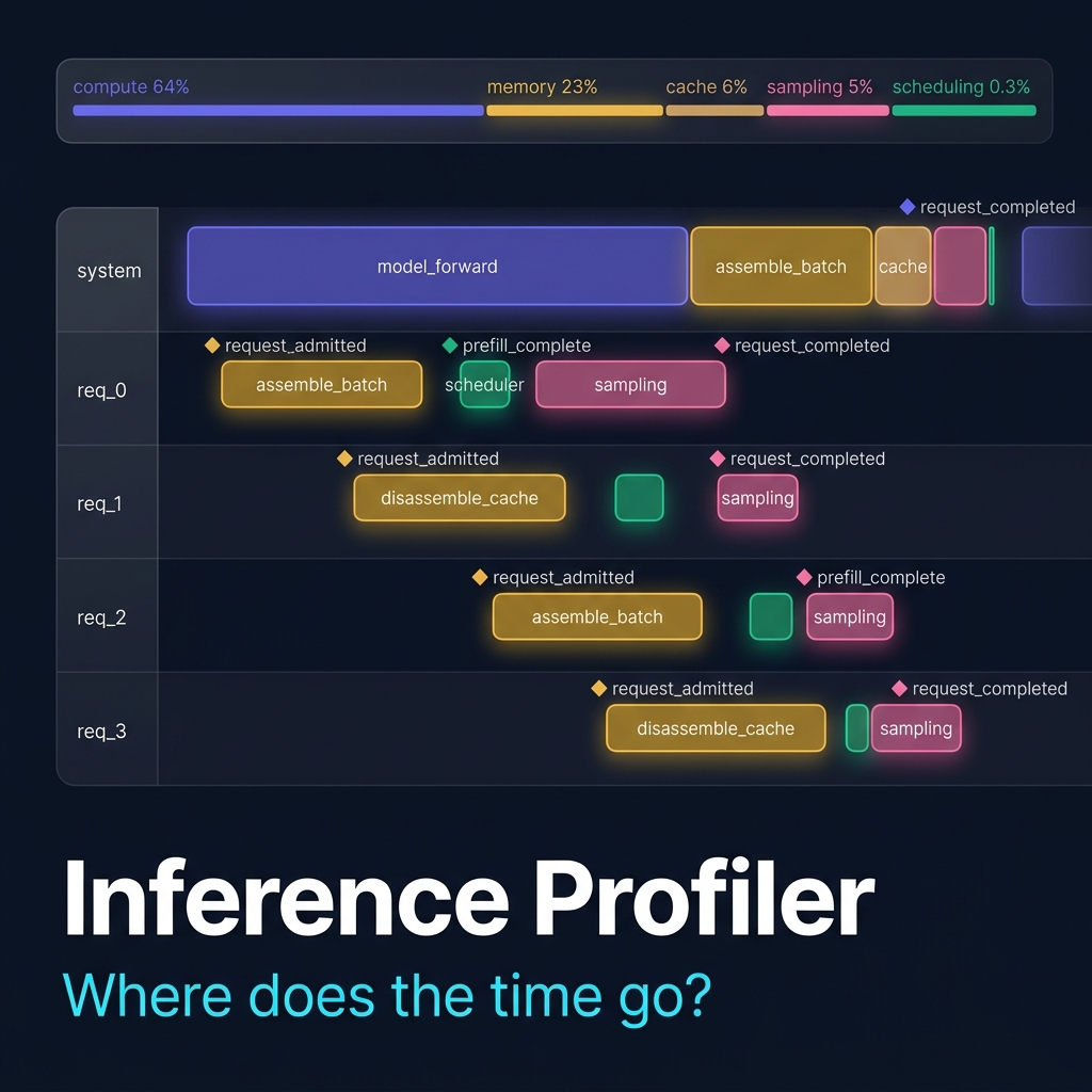
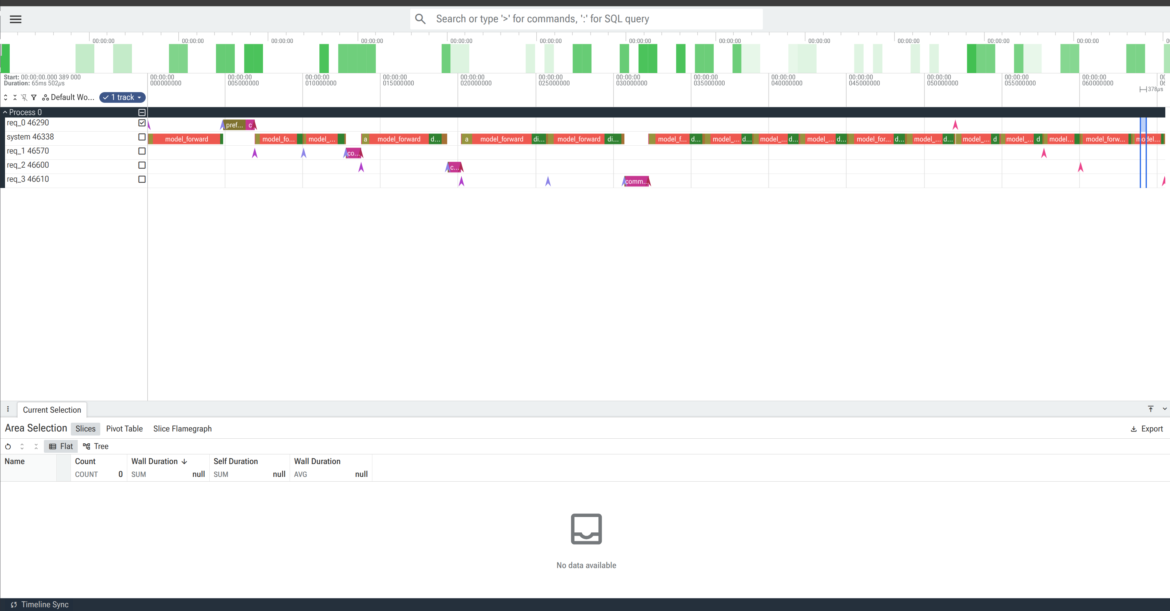
Here is the profiler’s output loaded in Perfetto, showing a 65ms trace of 4 concurrent requests through the interleaved engine. Each row is a swimlane: the system track shows model_forward spans (the transformer forward pass) dominating wall-clock time, while per-request tracks (req_0 through req_3) show lifecycle events (diamond markers for admission, prefill completion, and request completion) and request-scoped operations like commit_blocks for prefix cache writes. The staggered admission pattern is visible - each request enters one step after the previous one, and the timeline makes it clear how much time each request spends waiting for other requests’ prefill phases to complete.

Perfetto trace of 4 concurrent requests through the interleaved inference engine

The Problem with Existing Tools

Most inference profiling falls into one of two camps:

Too low-level. torch.profiler and CUDA profiling tools show kernel-level detail. You see aten::mm, aten::softmax, cudaLaunchKernel. But not “this is the prefill chunk for request 3” or “this is the scheduler deciding to preempt request 1.” The operations have no semantic meaning - you can’t tell which request a kernel belongs to, or whether a matrix multiply is part of attention or the feed-forward network.

Too high-level. Request latency dashboards show P50/P99 but not why a request was slow. Was it waiting for a batch slot? Was prefill chunked across multiple steps? Did another request’s long prefill starve it?

The profiler sits in the middle: it tracks semantic operations (scheduler decisions, prefill chunks, cache assembly, sampling) with wall-clock timing, tagged per-request.

Half 1: Python Instrumentation

The Span Data Model

Every profiled operation becomes a Span:

@dataclass
class Span:
    name: str                           # e.g., "attention_forward", "scheduler.schedule"
    category: str                       # e.g., "attention", "scheduling", "memory"
    start_us: int                       # microsecond timestamp (relative to trace epoch)
    end_us: int                         # microsecond timestamp (relative to trace epoch)
    request_id: Optional[str] = None    # which request this belongs to (None = system-level)
    metadata: dict = field(default_factory=dict)

The key design choice: every span carries an optional request_id. System-level operations (scheduling, model forward) have request_id=None. Request-specific operations (prefill chunks, sampling, lifecycle events) carry request_id="req_0". The timeline viewer uses this to place spans in per-request swimlanes.

The Trace Collector

A global singleton that accumulates spans during a profiled run:

class TraceCollector:
    def __init__(self):
        self.spans: list[Span] = []
        self.enabled: bool = False
        self._epoch_us: int = 0

    def begin_trace(self):
        self.spans = []
        self.enabled = True
        self._epoch_us = time.perf_counter_ns() // 1000

    def end_trace(self) -> list[Span]:
        self.enabled = False
        return self.spans

    def record(self, name, category, start_us, end_us, request_id=None, **metadata):
        if not self.enabled:
            return
        self.spans.append(Span(
            name=name, category=category,
            start_us=start_us, end_us=end_us,
            request_id=request_id, metadata=metadata,
        ))

All timestamps are relative to the trace epoch (the moment begin_trace() was called). This means the first span always starts near t=0, regardless of when the Python process started.

The enabled flag is the zero-overhead switch. When enabled=False, every record() call returns immediately without allocation. Production code can leave instrumentation in place with no cost.

Instrumentation Primitives

Three ways to add profiling to code, from least to most invasive:

1. Context manager - for wrapping inline blocks:

with trace_span("assemble_fused_batch", "memory", num_decode=3, chunk_size=14):
    batch_tokens, positions, past_kvs, mask, pads = assemble_fused_batch(
        decode_reqs, prefill_req, chunk_size
    )

The context manager calls trace._now() on entry, yields, calls trace._now() again on exit, and records the span. Metadata is passed as keyword arguments - num_decode=3 becomes {"num_decode": 3} in the span’s metadata dict, which the timeline tooltip displays on hover.

2. Decorator - for wrapping entire functions:

@profiled("model_forward", "compute")
def forward(self, idx, targets=None, pos=None, past_kvs=None):
    ...

3. Event marker - for instantaneous events (zero-duration spans):

trace_event("request_admitted", "lifecycle",
            request_id="req_0", prompt_len=14, cached_tokens=0)

Events appear as diamond markers on the timeline. They’re used for state transitions: request admitted, prefill complete, request done, preemption.

All three primitives are no-ops when trace.enabled is False.

What We Instrument

The interleaved prefill+decode engine has the most interesting profiling surface because a single scheduler step involves multiple operation types: scheduling, batch assembly, a fused forward pass, cache disassembly, and sampling - all serving multiple concurrent requests.

Here’s the instrumented interleaved_generate_profiled loop, showing where each span is recorded:

while not scheduler.is_done():
    # 1. Scheduling
    with trace_span("scheduler.schedule", "scheduling",
                    step=step, num_waiting=..., num_active=...):
        prefill_req, decode_reqs = scheduler.schedule(step)

    # 2. Batch Assembly
    with trace_span("assemble_fused_batch", "memory",
                    num_decode=len(decode_reqs), chunk_size=chunk_size):
        batch = assemble_fused_batch(decode_reqs, prefill_req, chunk_size)

    # 3. Forward Pass
    with trace_span("model_forward", "compute",
                    batch_size=B, seq_len=T, prefill_chunk=chunk_size):
        logits, _, new_kvs = model(batch_tokens, pos=positions, ...)

    # 4. Cache Disassembly
    with trace_span("disassemble_fused_cache", "memory", num_requests=...):
        disassemble_fused_cache(all_reqs, new_kvs, num_new_tokens)

    # 5. Sampling
    with trace_span("decode_sampling", "sampling", num_decode=...):
        probs = F.softmax(logits[:len(decode_reqs), -1, :], dim=-1)
        idx_next = torch.multinomial(probs, num_samples=1)

    # 6. Lifecycle events
    trace_event("request_completed", "lifecycle", request_id="req_0", ...)

Each scheduler step produces 5-7 spans. Over a typical 17-step run with 4 requests, this generates ~110 spans, enough to see the full pipeline behavior without being noisy.

The categories are chosen to match the conceptual phases of inference:

Category	Color	Spans	What it captures
compute	Indigo	`model_forward`	The transformer forward pass (attention + FFN)
memory	Amber	`assemble_fused_batch`, `disassemble_fused_cache`	Cache padding, concatenation, scatter-back
scheduling	Emerald	`scheduler.schedule`	Admission, preemption, batch selection
sampling	Pink	`decode_sampling`, `prefill_first_token`	Softmax + multinomial per-request
cache_management	Teal	`commit_blocks`	Writing completed KV blocks to the prefix cache
lifecycle	Slate	`request_admitted`, `prefill_complete`, `request_completed`	Instantaneous state transitions
prefill	Blue	`prefill_chunk`	Marks which tokens were prefilled this step

The Output Format: Chrome Trace Events

The profiler exports spans in Chrome Trace Event Format - a JSON schema originally designed for Chrome’s chrome://tracing viewer and now supported by Perfetto.

Each span becomes either an “X” (complete) event or an “i” (instant) event:

{
  "name": "model_forward",
  "cat": "compute",
  "ph": "X",
  "ts": 755,
  "dur": 4329,
  "pid": 0,
  "tid": "system",
  "args": {
    "step": 0,
    "batch_size": 1,
    "seq_len": 14,
    "num_decode": 0,
    "prefill_chunk": 14
  }
}

The key design choice: tid (thread ID) is set to the request ID. Chrome and Perfetto use tid to group events into rows. By mapping tid to request_id, every request gets its own swimlane automatically - no custom viewer needed. System-level spans use tid: "system" and get their own row.

The export also embeds a summary block with per-category and per-request aggregates, which the React viewer uses for the breakdown bar and legend:

"summary": {
  "total_us": 65502,
  "total_spans": 110,
  "by_category": {
    "compute":     { "total_us": 42119, "pct": 64.3 },
    "memory":      { "total_us": 15074, "pct": 23.0 },
    "cache_management": { "total_us": 3668, "pct": 5.6 },
    "sampling":    { "total_us": 3191,  "pct": 4.9 },
    "scheduling":  { "total_us": 210,   "pct": 0.3 }
  }
}

The Profiled Engine: Duplication by Design

The profiler can’t simply import nanogpt-interleaving because that file has top-level training code that executes on import. So we use the same pattern as the eval harness: a self-contained profiled_engine.py that duplicates the model architecture, scheduler, and generate loop with instrumentation inlined.

This is deliberate. The alternative - monkey-patching functions at runtime - would let us instrument without duplicating code, but at the cost of fragile reflection, inability to instrument inside loop bodies, and unclear ownership of the instrumentation points. The duplication means the profiled engine is a standalone artifact: you can read it top-to-bottom and see exactly what’s instrumented and why.

The model architecture is byte-for-byte identical to nanogpt-interleaving.py. The only differences are:

Module-level globals are set via configure() instead of hardcoded constants
The generate function has trace_span and trace_event calls at each pipeline stage
The scheduler’s _maybe_admit and _maybe_preempt methods record lifecycle events

Half 2: The React Timeline Viewer

The frontend renders the trace as an interactive flame chart at the /profiler route.

Loading Traces

The page offers two ways to load a trace:

Drag-and-drop (or file picker) for custom traces
Bundled examples - pre-generated traces served from the app’s public directory

The useTraceData hook handles both paths. It parses the Chrome Trace Event JSON, filters for “X” and “i” events, groups spans by tid (swimlane), computes per-category aggregates, and returns structured data for the chart.

The SVG Timeline

The chart is an SVG element (not Canvas) because NanoGPT traces have ~100-500 spans, well within SVG’s performance budget, and SVG gives us built-in mouse event handling per-element.

Each request is a horizontal swimlane. The x-axis is wall-clock time in microseconds. Spans are colored rectangles positioned by (startUs, endUs):

Time (ms) →    0      10      20      30      40      50      60
              ├───────┼───────┼───────┼───────┼───────┼───────┤

system        ▓sched▓ ▓▓▓ memory ▓▓▓ ████ compute ████ ▓mem▓ ████ compute ████ ...

req_0         ◇admitted           ◇prefill_complete              ◇completed
                ████ commit ████              ██ sampling ██

req_1                  ◇admitted        ◇prefill_complete         ◇completed
                         ████ commit ████         ██ sampling ██

req_2                         ◇admitted      ◇prefill_complete     ◇completed

req_3                                ◇admitted     ◇prefill_complete ◇completed

Duration spans render as rounded rectangles. Instant events (lifecycle transitions) render as diamond markers. Spans wider than 50px get an inline text label. Spans narrower than 3px are clamped to 3px so they remain visible.

Hover Tooltips

Hovering over any span shows a tooltip with:

Span name and category (with a color swatch)
Duration (for non-instant events)
Request ID (for request-scoped spans)
All metadata key-value pairs from the args dict

For example, hovering over a model_forward span shows:

model_forward
Category    Compute
Duration    4.3ms
step        0
batch_size  1
seq_len     14
num_decode  0
prefill_chunk 14

This tells you: step 0 was a pure prefill step (no decode requests), processing 14 tokens for one request.

Click-to-Pin Detail Panel

Clicking a span pins a detail panel at the bottom of the page. This is useful for comparing spans: click a span to pin it, then hover over another span to see both.

Category Legend and Breakdown Bar

A color legend maps each category to its color. Below the toolbar, a proportional breakdown bar shows the time split visually:

████████████████████████████████████████░░░░░░░░░░░░░░░░░░░░░░░░░░░░
         compute (64%)              memory (23%)   cache(6%) sample(5%)

This immediately communicates the dominant cost.

Reading the Trace: What the Numbers Show

Running the profiler on 4 requests through the interleaved engine produces this breakdown:

Category	Time	% of total	Span count
compute	42.1 ms	64.3%	17 spans
memory	15.1 ms	23.0%	34 spans
cache_management	3.7 ms	5.6%	4 spans
sampling	3.2 ms	4.9%	20 spans
scheduling	0.2 ms	0.3%	17 spans
lifecycle	0.0 ms	0.0%	12 spans
prefill	0.0 ms	0.0%	6 spans

Compute dominates at 64%

Not surprising. The model forward pass (attention + FFN across 4 layers) is the core operation. Each model_forward span is 2-5ms depending on batch size and sequence length. The first forward pass (pure prefill of 14 tokens) takes ~4.3ms. Later steps with a fused batch of 3 decode requests + 1 prefill chunk are slightly shorter because the decode tokens are single-position.

Memory is the second-largest cost at 23%

This is the interesting finding. Nearly a quarter of the inference time is spent on cache assembly and disassembly - torch.cat to left-pad variable-length KV caches, torch.zeros to create padding tensors, and scattering results back to per-request storage.

This is exactly the overhead that paged attention was designed to eliminate. With paged attention, KV cache lives in fixed-size blocks in a shared pool, and attention kernels read directly from the pool via a block table. No padding, no concatenation, no scatter-back. The profiler quantifies the cost that paged attention saves.

Scheduling is nearly free at 0.3%

The scheduler’s _maybe_admit and _maybe_preempt methods take ~12 microseconds per step. This confirms that scheduling overhead is negligible compared to compute and memory - the scheduler is not a bottleneck. This is expected for a simple FCFS policy with 4 requests. With hundreds of concurrent requests and complex priority policies, scheduling cost would grow, and the profiler would show it.

Sampling is modest at 5%

Softmax + multinomial per decode step costs 150-200 microseconds. With 20 sampling spans across the run, this adds up to 3.2ms. Not dominant, but not trivial either. In production engines with large vocabularies (32K-128K tokens), sampling cost is proportionally much lower because the forward pass cost scales with model depth while sampling scales with vocabulary size.

Per-request latency

The summary also breaks down time by request:

Request	Latency	Prompt	Generated
req_0	52.0 ms	14 tokens	12 tokens
req_1	50.8 ms	16 tokens	12 tokens
req_2	46.3 ms	12 tokens	12 tokens
req_3	45.3 ms	17 tokens	12 tokens

Request 0 has the highest latency despite having a shorter prompt than requests 1 and 3. This is because req_0 is admitted first and must wait through all subsequent requests’ prefill phases before reaching its own decode steps. The timeline view makes this visible: req_0’s swimlane shows a long gap between its prefill_complete event and its first decode sampling span, during which other requests are being prefilled.

The Architecture Decision: Batch vs. Live

The profiler is a batch tool: run inference, produce a JSON file, load it in the viewer. We considered a live-streaming architecture (WebSocket from Python to React, spans stream in real-time) but rejected it for three reasons:

Complexity. Live streaming requires buffering, backpressure, partial rendering, and WebSocket lifecycle management. The batch approach is two independent halves with a simple JSON contract.
The educational value is the same. The simulation page already has step-by-step animation for teaching concepts. The profiler serves a different purpose: post-hoc analysis of real execution. You want to zoom, pan, and compare spans across the full trace - which requires the complete data upfront.
Perfetto compatibility. By outputting standard Chrome Trace Event JSON, users get two viewers for free (Perfetto and chrome://tracing) without needing to run the React frontend at all.

What This Enables

With the profiler in place, every future optimization becomes measurable at a granular level:

Before paged attention: “Memory operations take 23% of inference time.” After paged attention: “Memory operations dropped to 3%. The gather_kv_from_pool spans are 10x faster than assemble_batch_cache.”

Before CUDA graphs: “Each decode step takes 4ms eager.” After CUDA graphs: “Each decode step takes 3ms graph replay. The model_forward spans are uniformly shorter.”

Before speculative decoding: “17 forward passes for 48 tokens.” After speculative decoding: “8 verify passes for 48 tokens. Acceptance rate spans show 65% accept.”

The profiler doesn’t replace throughput benchmarks or the eval harness. It complements them by answering the question they can’t: not “how fast” or “how correct”, but “where does the time go?”

You can find the code in the profiler/ directory and the visualization at the /profiler route of the frontend, in my nanoGPT inference repository here.