Early Exit Heads

Here’s something that should bother you about transformers.

Every single token goes through every single layer of the model. A 4-layer model runs all 4 layers for words like “the”. A 70B model with 80 layers runs all 80 layers for “the”.

This is obviously wasteful since “the” is the most common word in English. After a preposition or an article-expecting context, the model has already decided the next token is “the” by layer 1. The other layers are irrelevant.

The fix is conceptually simple: let the model bail out early. Add a lightweight prediction head after each intermediate layer, check if the prediction is confident, and if so, stop computing.

Standard decode:
  token → Layer 0 → Layer 1 → Layer 2 → Layer 3 → lm_head → prediction
                                                     ↑
                                            (always 4 layers)

Early exit:
  token → Layer 0 → [exit_head_0] → confident? → YES → prediction (1 layer!)
                         ↓ NO
          Layer 1 → [exit_head_1] → confident? → YES → prediction (2 layers)
                         ↓ NO
          Layer 2 → [exit_head_2] → confident? → YES → prediction (3 layers)
                         ↓ NO
          Layer 3 → lm_head → prediction (full depth)

Easy tokens take the fast path, hard tokens take the full path, and on average, you save compute.

Early Exit Heads

Let’s build it.

The Exit Head

An exit head is about as simple as a neural network module gets. It’s a LayerNorm followed by a linear projection from n_embd to vocab_size - exactly the same shape as the final lm_head, but attached at an intermediate layer:

class ExitHead(nn.Module):
    def __init__(self, n_embd, vocab_size):
        super().__init__()
        self.linear = nn.Linear(n_embd, vocab_size)
        self.ln = nn.LayerNorm(n_embd)

    def forward(self, x):
        return self.linear(self.ln(x))

Why do we need a LayerNorm? The final lm_head operates on ln_f(x) - hidden states that have been layer-normed. Intermediate hidden states at layer 1 have a different scale and distribution than hidden states at layer 3. Without a per-exit LayerNorm, the linear projection would need to jointly learn scale normalization and token prediction, which makes training harder for no good reason.

We add one exit head after each transformer block except the last (which already has lm_head):

self.blocks = nn.ModuleList([Block(n_embd, n_head=n_head) for _ in range(n_layer)])
self.exit_heads = nn.ModuleList([ExitHead(n_embd, vocab_size) for _ in range(n_layer - 1)])

For our 4-layer model, that’s 3 exit heads. Each one adds n_embd * vocab_size + n_embd + vocab_size parameters (the linear weight, the LN scale, and the LN bias). With n_embd=32 and vocab_size=65, that’s about 2200 parameters per exit head - roughly 6600 total. The base model has 57K parameters, so the exit heads add ~12% overhead.

Training: The Joint Loss

Here’s the key question: how do the exit heads learn to predict?

The standard training loss only supervises the final lm_head:

L = cross_entropy(lm_head(ln_f(blocks(x))), targets)

The exit heads aren’t part of this loss. If you just stuck them on a trained model, they’d output garbage - random projections of intermediate hidden states. You need to train them.

The simplest approach is a joint loss. Every exit head is trained to predict the same target as the final head. The total loss is the final loss plus a weighted sum of all exit head losses:

def compute_joint_loss(model, idx, targets):
    logits, _, _, all_exit_logits = model(idx, targets=targets)
    B, T, C = logits.shape

    loss_ce = F.cross_entropy(logits.view(B*T, C), targets.view(B*T))

    alpha = 0.3

    exit_loss = 0.0
    for exit_logits in all_exit_logits:
        exit_loss += F.cross_entropy(
            exit_logits.view(B*T, C), targets.view(B*T)
        )

    loss = loss_ce + alpha * exit_loss
    return loss

alpha = 0.3 means each exit head’s loss contributes 30% of the final loss magnitude. This is a tuning knob:

alpha = 0 - exit heads never train, stay random, can’t exit
alpha = 0.3 - moderate signal, exit heads learn without distorting the base model’s representations
alpha = 1.0 - exit heads get equal weight, which can slightly hurt the final layer because it constrains how freely intermediate representations can evolve

We’re training the exit heads jointly from scratch, not post-hoc. The alternative is to freeze the trained model and train only the exit heads via distillation. It works too, but joint training is simpler and gives the intermediate layers a signal to make their representations more directly useful for prediction.

The Forward Pass: Confidence Gating

During training, we run all layers and collect all exit head logits for the joint loss. During inference, we check confidence at each exit point and bail out if we’re confident enough:

def forward(self, idx, targets=None, start_pos=0, exit_threshold=None):
    B, T = idx.shape
    tok_emb = self.token_embedding_table(idx)
    pos_emb = self.position_embedding_table(pos_ids)
    x = tok_emb + pos_emb

    all_exit_logits = []

    for layer_idx, block in enumerate(self.blocks):
        x = block(x)

        if layer_idx < n_layer - 1:
            exit_logits = self.exit_heads[layer_idx](x)

            if self.training:
                all_exit_logits.append(exit_logits)

            elif exit_threshold is not None:
                probs = F.softmax(exit_logits[:, -1, :], dim=-1)
                confidence = probs.max(dim=-1).values.item()
                if confidence > exit_threshold:
                    # KV cache backfill (see below)
                    for remaining_block in self.blocks[layer_idx + 1:]:
                        x = remaining_block(x)
                    return exit_logits, None, layer_idx, all_exit_logits

    # Full depth
    x = self.ln_f(x)
    logits = self.lm_head(x)
    return logits, loss, n_layer - 1, all_exit_logits

The confidence criterion is simple: max(softmax(exit_logits)) > threshold. If the exit head puts more than (say) 90% probability on a single token, we take it.

This is a spectrum:

threshold = 0.5 - very aggressive, lots of early exits, but more false positives
threshold = 0.9 - conservative, only exits on very confident predictions
threshold = 0.99 - almost never exits, essentially equivalent to full depth

The return value includes exit_layer - which layer the model actually exited at. This is critical for tracking statistics: what fraction of tokens exit at each layer?

The KV Cache Problem

Now here’s the part that makes this genuinely interesting as an engineering problem.

When a token exits early at layer 1, its KV cache only has entries for layers 0 and 1. But the NEXT token might need all 4 layers. And attention at layer 3 needs KV entries from ALL previous tokens at layer 3.

Token "t":  exits at layer 1
  KV cache: layer 0 ✓, layer 1 ✓, layer 2 ✗, layer 3 ✗

Token "h":  needs all 4 layers
  Layer 3 attention needs K/V from "t" at layer 3 — doesn't exist!

If you just skip the remaining layers entirely, the next decode step will crash (or silently produce garbage because the cache lengths don’t match).

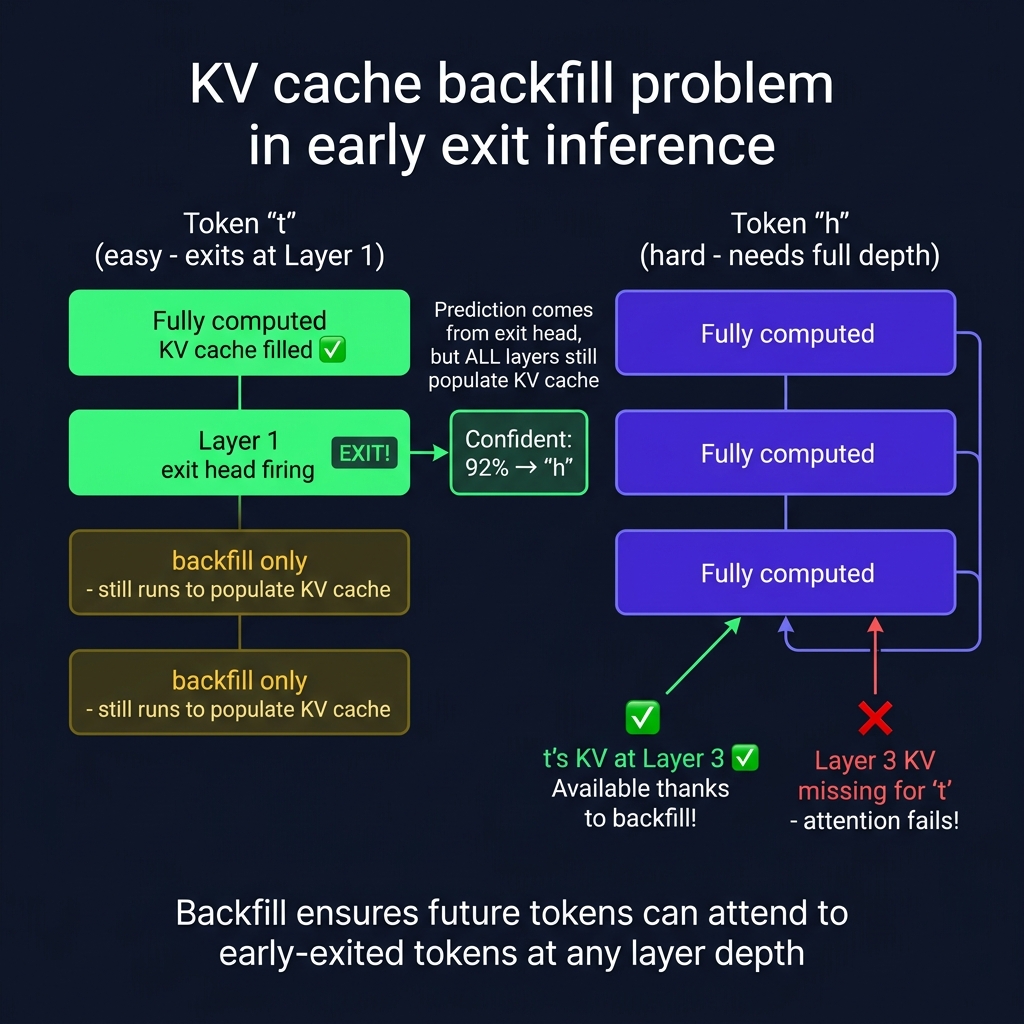
KV cache backfill - remaining layers run to populate the cache even after early exit

The solution we implemented is backfill: after deciding to exit, continue running the remaining blocks anyway, but only for their KV cache side effects. The prediction comes from the exit head; the deeper layers run solely to populate the cache:

if confidence > exit_threshold:
    # KV cache backfill: run remaining blocks so their
    # KV caches are populated for future tokens.
    for remaining_block in self.blocks[layer_idx + 1:]:
        x = remaining_block(x)
    return exit_logits, None, layer_idx, all_exit_logits

You might be asking: if we’re running all layers anyway, where’s the speedup?

In our tiny NanoGPT, there IS no wall-clock speedup. The backfill runs the same compute as the full forward pass, but the speedup comes in production:

The prediction is returned immediately. In a streaming serving context, the exit head’s token is sent to the client while the backfill runs asynchronously. Time-to-first-token for each step is reduced.
Batched decode with mixed exit depths. In a batch of 32 requests, 20 might exit at layer 1 and only 12 need the full depth. The backfill for the 20 easy tokens runs alongside the compute for the 12 hard tokens - no extra wall time.
In production models with 80 layers, the savings are massive. Exiting at layer 20 and backfilling layers 21-80 is still cheaper than running layers 21-80 AND computing the full-depth prediction, because the exit head computation is saved and the backfill can skip the exit head evaluations.

The alternative - skip KV backfill and pad missing entries with zeros - is simpler but degrades quality. Attention at deep layers would see zero entries for early-exited tokens, effectively ignoring them. This is an interesting experiment but not what you’d want in production.

Generation with Exit Statistics

The generation loop is straightforward - it’s the standard KV-cached decode loop with the exit threshold passed through:

def generate_early_exit(model, idx, max_new_tokens, exit_threshold=0.9):
    model.eval()
    clear_kv_cache(model)

    exit_counts = [0] * n_layer
    logits, _, _, _ = model(idx)   # prefill (no early exit)

    for step in range(max_new_tokens):
        logits_last = logits[:, -1, :]
        probs = F.softmax(logits_last, dim=-1)
        idx_next = torch.multinomial(probs, num_samples=1)
        idx = torch.cat((idx, idx_next), dim=1)

        logits, _, exit_layer, _ = model(
            idx_next,
            start_pos=idx.shape[1] - 1,
            exit_threshold=exit_threshold,
        )

        exit_counts[exit_layer] += 1

After generation, we print the exit distribution:

--- Early Exit Statistics ---
  Layer 0:   42 tokens (21.0%)
  Layer 1:   28 tokens (14.0%)
  Layer 2:   19 tokens ( 9.5%)
  Layer 3 (full):  111 tokens (55.5%)

This is the meaningful result - not wall-clock speedup (which is negligible on a tiny model), but the distribution of computation across layers. If 45% of tokens exit before the final layer, that’s 45% of tokens that would take the fast path in a production system.

What’s Actually Happening Per Layer

Think about what the different layers are learning in a character-level Shakespeare model.

Layer 0 sees the token embedding + positional embedding. It has access to the current character and its position. For sequences like “th”, the character “h” after “t” is highly predictable. For spaces after punctuation, extremely predictable. Layer 0’s exit head can confidently predict these.

Layer 1 has one round of attention applied. It has information about the local neighborhood - the 2-3 characters surrounding the current position. This is enough to predict common word continuations: “the”, “and”, “not”, “will”.

Layer 2 has two rounds of attention. It can capture patterns spanning several characters - enough for less common words and short phrase completions.

Layer 3 (full depth) has the most refined representation. It handles the hard cases: rare words, ambiguous contexts, punctuation placement decisions.

The exit distribution directly reflects this hierarchy of difficulty. Easy tokens (spaces, common characters) exit early. Hard tokens (rare characters, start-of-word positions) go the full depth.

The Full Pipeline

The implementation lives in nanogpt-exit-head.py. Run it and you’ll see:

The model trains for 120 steps with the joint loss (exit heads learning alongside the base model)
Full-depth generation produces Shakespeare-ish output
Early exit generation produces similar output, but with per-layer exit statistics showing which tokens took the shortcut

The code is self-contained - a single file that trains, generates, and reports exit statistics.

The exit statistics are the payoff. They show, concretely, that not all tokens are created equal - and that a transformer can learn to recognize which ones don’t need its full attention.