Pruning DeepSeek V4 Flash 0731 To Save 21GB: A Comprehensive Guide
I have been working for the past few months with DeepSeek V4 Flash 0731 to primarily run my stock-research bot on my single DGX Spark. It has been amazing to automate the previously tedious research process and have well-researched stock reports deposited into my custom Discord channel every morning.

But my DGX Spark can run several local models at once, so why use only one?
I have always wanted to create a model router that can intelligently select the best local model for a given task. My idea was to use DeepSeek to serve as a high reasoning model while a smaller model like Qwen could handle simpler tasks.
The problem was that DeepSeek was a very large model which took up most of my Spark’s 128 GB of memory. To fit a second 27B model with enough KV cache to be useful, I had to make DeepSeek much smaller.
Since DeepSeek is a mixture of experts model, I wanted to know if I could remove the experts that my bot rarely used. Further quantization made no sense since I was already using a heavily quantized EXL3 model.
Here are the original model specs:
| Item | Value |
|---|---|
| Base model | deepseek-ai/DeepSeek-V4-Flash 0731: 284 B parameters; 240.7 B after the REAP prune |
| Layers | 43 MoE layers, hidden size 4096, plus 3 mtp layers |
| Routed experts (K) | 216 per layer (256 before the REAP prune) |
| Experts per token (top-k) | 6 routed + 1 shared |
| Routing, layers 0 to 2 | Hash: a fixed token-to-expert table (ffn.gate.tid2eid) |
| Routing, layers 3 to 42 | Learned router: sqrtsoftplus score + ffn.gate.bias, top-6, weights normalized |
| One expert | 3 × 4096 × 2048 = 25.2 M parameters = 9.47 MB at 3.0 bpw |
| Expert storage | EXL3 3.0 bpw trellis; 12 tensors per expert; one 2.05 GB file per layer |
| Other weights | Attention, shared experts, embeddings, head: FP8/BF16, about 7 B parameters, 18 GB |
| Size on disk | 106.8 GB (99.5 GiB) |
| Draft model | DSpark: a separate folder with 64 MTP experts |
REAP pruning (Router-weighted Expert Activation Pruning) is a one-shot method from Cerebras. It runs a calibration dataset through the model and gives each expert a score: the router’s gate weight times the size of the expert’s output, averaged over the tokens that the router sends to that expert. REAP then removes the lowest-scoring experts in each layer, and the model needs no retraining. Here, it removed 40 of the 256 experts in each layer.
DSpark is a speculative decoding method from DeepSeek. A small draft model proposes a block of tokens in one parallel pass, and a light “Markov head” links each draft token to the token before it. The full model then checks the whole block in one pass and keeps the tokens that it agrees with.
EXL3 is the weight format of ExLlamaV3, an open-source library by turboderp for quantizing LLMs and running them on local GPUs. Here, the routed experts use 3.0 bits per weight. To learn more, start with the EXL3 section of the ExLlamaV3 README.
EXL3 makes pruning cheap: each expert has its own 12 tensors, so a prune can copy or drop them byte for byte, with no new quantization. The 12 tensors are three matrices (w1, w2, w3), each in four parts (trellis, suh, svh, mcg). One file holds the experts of one layer.
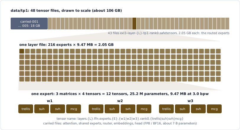
The weight files. The width of each file in the top strip is to scale. The 43 layer files hold the routed experts, about 88 GB of the 106 GB. Each step down zooms in: one layer file, then one expert.
The key idea of this project was that an MoE model has two separate levers:
- K, the number of routed experts in each layer, controls memory. The server loads all K experts, so a smaller K frees memory. It saves almost no time, because each token still reads 6 experts.
- Top-k, the number of experts that each token uses, controls speed. Memory bandwidth (about 273 GB/s) limits the decode on the Spark, so fewer bytes per token give more tokens per second. It saves no memory, because all K experts stay loaded.
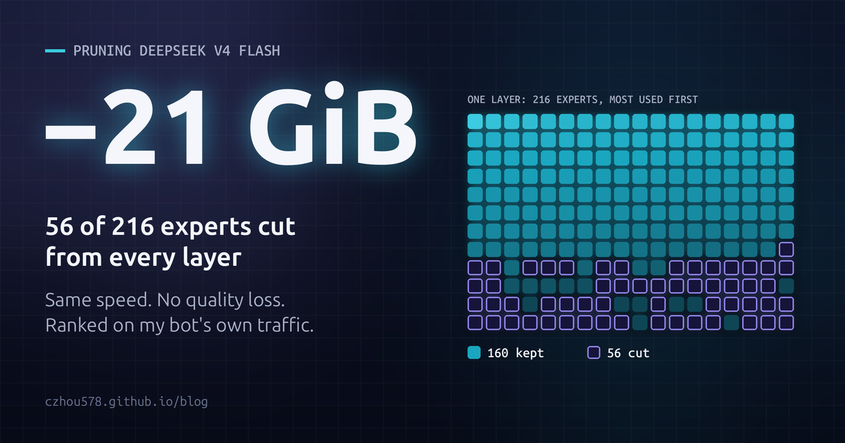
How far did K have to go? The second model of my router needed memory too, so I set a cap: the loaded DeepSeek weights had to stay at or below about 72 GiB. The stock model loaded 95.4 GiB, and each expert slot (one expert in every layer) cost about 0.42 GiB. So I had to drop about 56 slots: 95.4 − 56 × 0.42 ≈ 72 GiB. That left 216 − 56 = 160 experts per layer, so my target was K 160.
Each decode step with the DSpark draft checked 6 tokens: 5 draft tokens and 1 more. In each layer, a decode step read every expert that any of its 6 tokens picked. At K 216 and top-k 6, that was about 34 experts per layer: 13.7 GB per step, plus about 7 GB of static weights. If I cut K to 160, the count would only drop to about 33, because 6 tokens × 6 experts can never read more than 36. If I cut top-k to 5, it would drop to about 28.
So a smaller K alone would free memory but not speed up the decode. Only a smaller top-k could do that.
Building the baseline
I started by building a harness that could tell a real loss from run-to-run noise at three levels of cost.
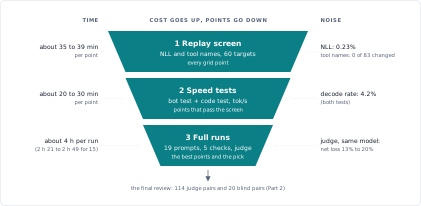
The three levels. The left side gives the time per test point, and the right side gives the noise between two runs of the same model. A change counted only if it was larger than the noise of its level.
The harness read my bot’s own history: 57 recorded sessions with 2,747 messages. Most of the text was tool output, such as SEC filings, web pages and price tables. A script tagged each session with its skill and reserved about 30% of the sessions for the tests. The rest became calibration data for the expert rank that I built later.
Level 1: the replay screen
The replay screen sent a recorded context up to an assistant turn, with that recorded turn as the last message:
system     You are a stock-research assistant for my portfolio.

user       Give me an update on ACME after its earnings.

assistant  [tool call] get_filing(ticker="ACME", form="10-Q")
tool       ...Revenue was $4.1 billion, up 12% from a year ago...

assistant  ACME's revenue rose 12% to $4.1 billion.    <- the recorded turn: the screen scores this one
A simplified example. The company, the tool and the numbers are made up.
vLLM returned the log-probability of every token in this prompt, and the screen kept only the tokens of the last turn. For each token, the question was: after everything before it, how likely did the model find the token that the stock model actually wrote?
The screen turned these probabilities into one score: the NLL (negative log-likelihood) per token, which is the mean of −ln p over the tokens of the turn. A token that the model expects (p near 1) adds almost nothing, and a surprising token (p near 0) adds a lot. So a lower NLL means that the model finds the recorded reply more likely.
| Token in the recorded turn | p, stock model | p, over-pruned model |
|—|—|—|
| ` rose | 0.80 | 0.75 |
| 12 | 0.97 | 0.70 |
| 4.1` | 0.95 | 0.60 |
| NLL per token (mean of −ln p) | 0.10 | 0.39 |
The stock model copies “12” and “4.1” from the tool result confidently. An over-pruned model that lost that skill is less sure, so its NLL goes up. A model passed the replay screen only if its NLL rose by at most 3%, measured over all 45,690 tokens of the 60 targets (the recorded turns that the screen scored).
One session gave more than one target, because the screen scored several of its assistant turns. In the ACME example, the tool call get_filing(...) is also a target: there, the prompt stops after the user message and that tool call. For each tool call in a target, the screen also checked the tool name. Every token of get_filing had to be the model’s first choice, so that the model would call the same tool if it wrote the turn itself. The 60 targets held 83 tool calls, and this check gave the “tool names” score later in the post, such as 77 of 83.
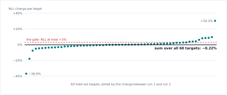
How I measured the noise floor. Each dot is one target: the change of its NLL from run 1 to run 2 of the same model. Single targets moved by up to 37% (median 1.6%), but the sum over all 60 targets moved by only 0.23%. So the gate used the total, never a single target or skill.
Level 2: the speed tests
The speed tests measured the decode speed in tokens/s.
The bot test sent the context of 10 held-out sessions up to the final report turn and decoded up to 1,024 tokens.
The code test was the server repo’s own benchmark: 5 fixed code prompts of 512 tokens, with thinking off. Each test did one warm-up run and then measured runs.
I ran both tests 5 times on the stock model. The bot test gave 33.64 tok/s and the code test 38.86 tok/s. The spread was 1.42 and 1.65 tok/s: 4.2% for both.
The tests also read the draft acceptance from the vLLM metrics: 2.25 accepted tokens per draft on the bot test and 2.67 on the code test.
Level 3: the full runs
The full runs answered whether the bot still did its job. The e2e (end to end) runner started one docker container per prompt and ran the bot’s own agent loop with live tools.
The prompts were the first messages of the 18 held-out sessions, plus the daily-report cron job: 19 bot prompts (the first runs used 15). One run of 19 prompts took about 4 hours.
Each run then went through five automatic checks:
- Tool-call validity. Every tool call that the model wrote had to parse. The server’s
deepseek_v4parser read each call, and one bad call would break a step of the agent loop. - Call order. The
stock-updateskill had to send its two writes and then the save, all in one message. This showed that the model still followed a multi-step instruction exactly. - Report marker. The final reply had to end with
[[report:FILE]], and the file that it named had to exist. - Takes JSON. The daily report wrote its takes to a JSON file. That file had to pass the bot’s own validator.
- Number fidelity. Each number in the final report had to appear in a tool result of the same session. For a stock bot, this is the important check: a pruned model must not invent a price or a revenue figure.
A pairwise LLM judge read the prompt and two final reports, without the model names. It answered A, B or tie. It judged each pair twice with the order swapped, and two different answers counted as a tie.
Using DeepSeek as its own judge
The judge was not a separate model. It was DeepSeek itself: the stock model on my live server. But a model that grades its own kind of answers brings risks.
- Self-preference. The judge could prefer reports in its own style, so it could favor the stock model. This bias worked against the pruned model. If the pruned model in this case still did not lose, the result held.
- Position bias. Without thinking, the judge picked position A in both orders for 9 of 15 pairs. The judge then thought before it answered, and each pair ran in both orders. A win or a loss counted only if it survived the swap.
- Noise. Two runs of the same stock model already gave a net loss of 13% to 20%. So in the full runs, the judge only reported and did not gate.
The gates
Here are the gates (requirements) of all three levels. A test point had to pass the gates of one level before it went to the next:
| Level | Metric | Gate |
|---|---|---|
| Replay screen | NLL per token, 60 targets | At most +3%: 13 times the noise floor |
| Replay screen | Next tool name | At least 98% of the baseline: 76 of 83 passes, 75 of 83 fails |
| Speed tests | Decode tok/s, bot test and code test | A change counted only above 4.2% |
| Full runs | Tool-call validity | 100%, no new failures |
| Full runs | Call order, report marker | No new failures |
| Full runs | Takes JSON | No missing or invalid file |
| Full runs | Number fidelity | Run share at most 1.5 points above the baseline; one prompt at most 5 points |
| Full runs | LLM judge | No gate: it reported only |
Each test boot stopped my live bot. So the test scripts had two safety rules in code: a memory watch stopped a test when free memory ran low, and the script always restored the live server at the end.
Finding the right size
I tested each size with a mask before I changed any weight file. The mask edited only the small routing tensors: the router never picked a dropped expert, but the server still loaded all 216. So I could test K 192, 176 and 160 cheaply, with no rewrite of the 43 expert files.
How it works in layers 3 to 42
Each dropped expert got a very large negative bias: gate.bias = -1e4. The router added the bias only to choose the top-6, so it never picked a dropped expert. The weights came from the scores without the bias.
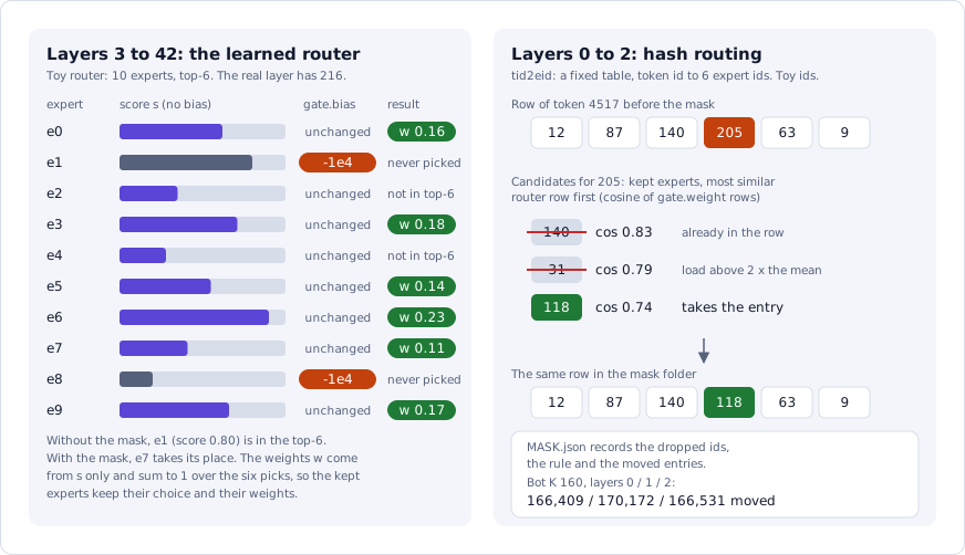
The mask in the two kinds of layer. Left: a toy router with 10 experts shows how a bias of −1e4 removes e1 from the top-6 and lets e7 in. The kept experts keep their scores, so their weights do not change. Right: a toy row of the hash table. The dropped expert 205 moves to the most similar kept expert that passes the two rules. The ids and scores are examples. The counts at the bottom come from MASK.json of the bot K 160 mask.
How it works in layers 0 to 2
DeepSeek V4 doesn’t use the score test in its first 3 layers: it uses a fixed table, ffn.gate.tid2eid, that maps each token id to 6 experts.
tid2eid, layer 0 (made-up ids)
  token 4516  →  [  3, 190,  44,  71, 158,  20]
  token 4517  →  [ 12,  87, 140, 205,  63,   9]
  token 4518  →  [101,   6, 177,  39, 212, 130]
  ...
For token 4517, layer 0 always runs these 6 experts, in every sentence. The bias trick from layers 3 to 42 does not work here: the table sends the token’s work to its experts, whatever their bias is.
The mask tool edited this table instead. Each entry for a dropped expert moved to the kept expert with the most similar router row. That kept expert had to pass two rules:
- It was not already in the same row.
- Its load stayed below twice the mean. Otherwise a few “central” experts would take the slots of many dropped experts. Without this rule, one expert got 12 times the median load at K 160.
before:  token 4517  →  [12, 87, 140, 205, 63, 9]     205 is dropped
         candidates: 140 (already in the row), 31 (load too high), 118 (OK)
after:   token 4517  →  [12, 87, 140, 118, 63, 9]
Exactness check
I read the vLLM code: the router adds the bias only to choose the experts, and it holds the bias in FP32, so −1e4 fits.
But one part of the routing ran purely in a CUDA kernel with no source code in the server image, so I tested the routing directly.
-
I booted the mask with routed-expert capture on, so that each reply listed the experts that each token used in each layer.
-
I sent four short prompts.
-
The test passed only if no dropped expert appeared in layers 3 to 42, and the rows of layers 0 to 2 matched the mask’s table.
On the bot K 160 mask, the router made 0 picks of a dropped expert over 71,583 tokens in all 43 layers.
Results
For the first masks, I used the public REAP rank: the same expert scores that made the original prune from 256 to 216 experts. For a mask with K experts, the mask tool dropped the 216 − K lowest-ranked experts of each layer. The top 32 experts of each of the two tool-call categories in the rank never dropped.
Then I ran each mask through the replay screen.
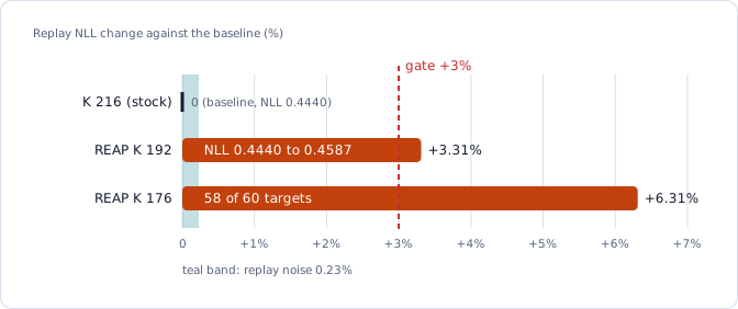
Both REAP masks failed the NLL gate. The replay screen on 60 held-out targets. K 176 ran on 58 of 60 targets, and its baseline was cut to the same 58.
Even the smallest cut failed. K 192 dropped 24 experts per layer, and its NLL rose from 0.4440 to 0.4587: +3.31%, just over the gate. K 176 dropped 40 experts per layer, and its NLL rose by 6.31%, about twice as much. The change at K 192 was 14 times the 0.23% noise floor, so it was a real loss.
The tool names held at both sizes: 78 of 83 at K 192, and 74 of 80 at K 176 (its 58 targets had 80 tool calls). The masked model still picked the right tools, but it found the bot’s replies less likely.
I stopped there, because the REAP rank could not take me to the size that I needed.
Why did REAP do so badly? Its rank came from code, math, science and tool-call data. My bot read earnings reports, SEC filings and web pages, so the REAP rank dropped some experts that my bot actually used. The next step was to rank the experts on my bot’s own traffic.
Rank experts on my bot’s traffic
First, I booted the unchanged model, with all 216 experts, in a capture mode. vLLM’s Model Runner V1 let me define a capture flag, --capture-return-routed-experts. With this flag, each reply listed the experts that the router picked for each token in each layer.
Next, a Python script sent the 34 segments of the calibration split to the model. If the rank and the test had used the same sessions, the replay screen would have graded the rank on the data that made it, skewing results.
Each request held the recorded context up to the last target turn, as in the replay screen, and the server wrote only one new token. Before that token, it read the full prompt through all 43 layers, and the router picked 6 experts for every prompt token. This read (prefill) processes all tokens in parallel, so it is much faster than writing tokens one at a time. It also gives the same routing as real use, because the router’s choice for a token depends only on the tokens before it. So 34 requests gave the expert choices for 2,023,990 tokens of real bot traffic.
The script then counted how often each of the 216 experts appeared in each layer, which gave 43 rows of 216 counts.
The shared prefix counted only once. Every request started with the same system prompt and tool definitions. If the script had counted them in all 34 requests, the experts that read the system prompt would have gotten 34 times their real weight. This is how 2,023,990 prompt tokens became 1.75 M counted tokens.
Finally, the script wrote the rank to expert_rank_bot.json: for each layer, all 216 experts, most used first.
The mask tool read this file the same way it read the REAP rank: for a mask with K experts, it dropped the 216 − K experts at the bottom of each layer’s list.
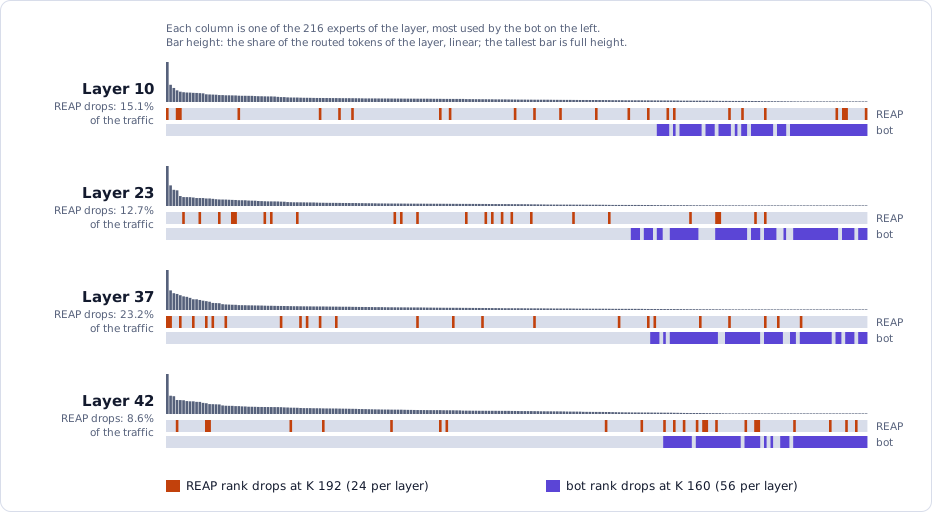
Four layers, expert by expert. The bars show how often my bot’s router picked each expert, most used on the left. The violet drops of the bot rank sit at the right end, in the tail that the bot hardly used. A few gaps there are the protected tool experts, which never dropped. The orange row marks the experts that the REAP mask dropped at K 192: some were among the most used experts of the layer. Layer 37 had the largest REAP share of the 40 layers.
Before I booted any new mask, I compared the two ranks on the capture data. The question was simple: how much of my bot’s routing went to the experts that each mask dropped? The less traffic the dropped experts carried, the less the bot would notice that they were gone.
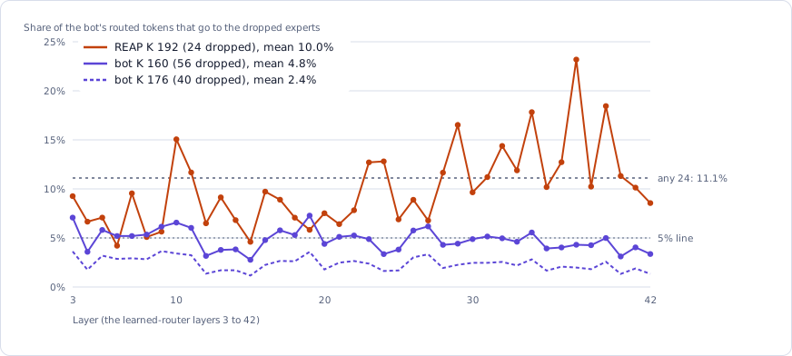
The REAP rank dropped more of the bot’s traffic with 24 experts than the bot rank did with 56. For each learned-router layer, the share of the bot’s routed tokens that went to the dropped experts of each mask. The dotted line marks the share of any 24 experts (24 of 216 = 11.1%).
The REAP mask at K 192 dropped only 24 experts per layer, but they carried 10.0% of my bot’s routed tokens on average, and 23.2% in layer 37. So for my bot, the REAP rank was barely better than a random choice of 24 experts, which would carry 11.1%.
The bot rank did much better. Its 40 least used experts carried 2.4% of the routing, and no layer went above 5%. Even its 56 least used experts carried only 4.8% on average (7.3% at most), although 17 of the 40 layers went above 5%. So the bot rank dropped more than twice as many experts as REAP, and still removed less than half as much of my bot’s traffic.
Results
Then I built the two bot-rank masks, K 176 and K 160, and ran them through the replay screen. The table also shows the baseline and the REAP mask at K 192. “Answer top-1” is the share of answer tokens that the model ranks first: how often its first choice is the token that the stock model wrote.
| Rank | K | NLL | NLL change | Answer top-1 | Tool names | Replay gates |
|---|---|---|---|---|---|---|
| none | 216 | 0.4440 | 0 | 91.40% | 77 of 83 | Baseline |
| REAP | 192 | 0.4587 | +3.31% | 91.08% | 78 of 83 | Fail |
| bot | 176 | 0.4453 | +0.29% | 91.24% | 77 of 83 | Pass |
| bot | 160 | 0.4501 | +1.37% | 91.23% | 78 of 83 | Pass |
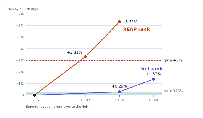
The bot rank moved the whole curve down. Replay NLL change against K for both ranks, at top-k 6. The bot rank at K 160 dropped 56 experts and cost less than half of the REAP rank at K 192, which dropped 24.
Both bot-rank masks passed the replay screen. K 176 cost +0.29%, close to the 0.23% noise floor. K 160 cost +1.37%, less than half of the +3% gate, and it was the size that I needed.
A pass here was a pass of the replay screen only. The replay targets came from the same weeks of traffic as the capture, so traffic of a new kind could use other experts.
Fewer experts per token
The problem now was that the DSpark draft was designed to work with the full K = 216 model, not with anything pruned.
When I ran the bot K 160 mask with the draft, the acceptance dropped from 2.25 to 2.09 tokens in the bot test and from 2.67 to 2.45 in the code test.
A smaller K could not win this back, because each token still read 6 routed experts.
So I cut top-k.
The top-k tool
My tool topk_checkpoint.py copied a mask folder and changed the number of experts per token. It changed no expert weights. vLLM reads top-k from one number in config.json, num_experts_per_tok, so the tool set that number to the new top-k. In every layer, top-k 5 meant the same thing: each token lost the weakest of its 6 experts.
In layers 3 to 42, the config change was enough. The router now took its top 5 in place of its top 6. vLLM then renormalized the weights of the 5 kept experts, so they added up to the same total as the 6 did. The mask bias still kept the dropped experts out.
Layers 0 to 2 needed more work. vLLM expects the tid2eid table to have one column for each expert of a token, so (129,280, 5) now. The file still held 6 columns, so the boot would fail with a shape mismatch. The tool had to drop one id from each row.
The column position means nothing, so the tool dropped the id with the smallest router weight, the same rule as in the other layers. The real weight depends on the input to the layer, and attention mixes the earlier tokens into that input. One token id gets a different input in every sentence, but the table has only one row for it. The tool used an estimate: it put the token’s own embedding in place of the real input, and dropped the id with the lowest score.
token "price", layer 0 (made-up numbers)
row before:  [ 17,   92,  140,    5,  201,   63 ]
est. score:  [1.4,  0.9,  1.6,  0.5,  1.2,  1.1 ]
row after:   [ 17,   92,  140,       201,   63 ]   <- id 5 has the lowest score
By the same estimate, the dropped expert carried about 12 to 13% of a token’s routing weight in these layers. With 6 equal weights, each expert would carry 16.7%. Thus, the tool dropped a weaker expert than average, but not one with zero weight.
Then the tool wrote the new folder. It rewrote only the file with the 3 tables and linked the rest. A self-check confirmed that each new row held only ids from the old row, and that every other tensor had the same bytes as before.
Each boot loaded the new tables with no error, and the EXL3 runtime line showed topk=5. But layers 0 to 2 used an estimate, so only the replay screen could show the real cost.
Testing potential top-k values
I had three values to test: 6, 5 and 4. Before any test, I estimated that top-k 5 would decode about 9% faster than top-k 6, and top-k 4 about 21% faster. But each expert that a token lost would also cost some quality, and I could not predict how much.
I wrote down the rules for the pick before the test:
- Drop each point that fails a gate.
- From the rest, take the fastest point. Two speeds within the 4.2% noise count as equal.
- If two points have equal speed, take the smaller one.
Then a script tested three points in one night, from 2026-11-04 to 2026-11-05: bot K 160 at top-k 5, bot K 160 at top-k 4, and K 216 at top-k 5 with no mask. For each point, it booted the server, ran the replay screen and then the speed tests (the median of 3 runs per test). At the end, it restored my live server.
Results
The speed changes compare each point with the stock model.
| Rank | K | Top-k | NLL change | Tool names | Bot test | Code test | Acceptance (bot / code) | Result |
|---|---|---|---|---|---|---|---|---|
| none | 216 | 6 | 0 | 77 of 83 | 33.64 tok/s | 38.86 tok/s | 2.25 / 2.67 | Baseline |
| bot | 160 | 6 | +1.37% | 78 of 83 | 31.50 (−6.4%) | 35.67 (−8.2%) | 2.09 / 2.45 | Slower |
| bot | 160 | 5 | +2.27% | 79 of 83 | 33.98 (+1.0%) | 42.07 (+8.3%) | 2.10 / 2.76 | The pick |
| bot | 160 | 4 | +6.05% | 79 of 83 | 36.05 (+7.2%) | 42.78 (+10.1%) | 2.00 / 2.51 | NLL fail |
| none | 216 | 5 | +1.29% | 49 of 54 | – | – | – | Pass (35 targets) |
Top-k 4 was the fastest point, but its NLL change of +6.05% was twice the gate. So rule 1 dropped it.
Top-k 5 passed with room to spare: +2.27% against the +3% gate, and it still picked the right tools. Compared with top-k 6 at the same K 160, it decoded 7.9% faster in the bot test and 17.9% faster in the code test, for only +0.87% more NLL. Top-k 5 won back all the speed that the mask lost, and the rules picked it.
The acceptance column shows where that speed came from. In the bot test, the acceptance hardly changed from top-k 6 (2.09 to 2.10), so the gain there came from fewer bytes per token. In the code test, the acceptance also rose from 2.45 to 2.76, even above the 2.67 of the stock model, so the code test gained more.
The last row, K 216 at top-k 5 with no mask, answered one more question: did the mask make the top-k cut worse? The memory watch stopped this replay at 35 of 60 targets, and the speed tests did not run. So I compared the points on those 35 targets only. There, top-k 5 alone cost +1.29%, and the mask alone cost +1.24%. Both together cost +2.50%, about the sum of the two. So the two costs simply added up, and neither change made the other one worse.
Full runs and the final review
Before I cut any experts out of the files, the pick (bot K 160 at top-k 5) had to pass two more tests: the full runs, and a final review of its answers.
The full run on 2026-11-05 sent 15 bot prompts through the real agent. All 15 finished, and the boot log showed topk=5. Every check passed except the report marker on one prompt: the model wrote the full report in its reply, but saved no file. The stock model also skipped that save on 1 of 3 runs of the same prompt, so I counted it as a problem of the prompt, not of the model.
The final review: 114 judge pairs and 20 blind pairs
The replay screen and the checks caught broken behavior, but they did not answer the main question: were the answers still as good?
- 114 judge pairs. The LLM judge compared a report of the stock model with a report of the pick for the same prompt. I ran the stock model 3 times and the pick 2 times on all 19 held-out prompts, which gave 3 × 2 × 19 = 114 pairs.
- 20 blind pairs that I reviewed myself. A review page showed each pair as A and B, with no run names and in a random order. For each pair, I chose the better report or a tie.
I also ran 57 control pairs: each stock run against each other stock run.
If the two models were equal, each pair with a winner would be a coin flip. A sign test checked if the pick lost more pairs than chance allowed (p < 0.05). The pick would fail if the judge or my own review found a loss. No control was allowed to fail the same test.
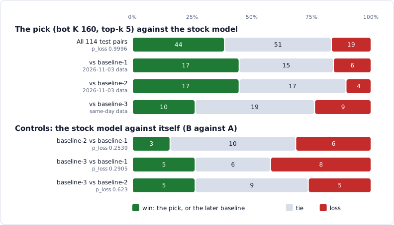
The judge found no loss, and the controls found no bias. Each bar shows the share of pairs, and the numbers are pair counts. Against the two older baselines, the pick had 34 wins and 10 losses. Against baseline-3, which ran on the same day as the new runs, it had 10 wins and 9 losses. In a control, a win is a win of the later baseline.
The pick passed all three rules:
- LLM judge, 114 pairs: 44 wins, 51 ties and 19 losses for the pick. The fail line was about 38 losses, so the judge found no loss.
- Controls, 57 pairs: No control failed the test in either direction, so the judge showed no bias toward one side.
- My blind review, 20 pairs: I preferred the pick in 9 pairs and the stock model in 6, with 5 ties. The pick would have failed only if I had preferred the stock model in 12 of the 15 decided pairs.
The judge and I agreed on only 9 of the 20 pairs, so it turned out the judge was a good check for “no loss” over many pairs, but not for a single pair.
I also read the answers for hard faults. Wrong numbers came up on both sides, so they did not separate the two models. Two faults of the pick looked like effects of the mask: a literal </s> in a broken sentence, and a call to a tool that did not exist. On 2026-11-06, I accepted these faults, and the pick passed.
Lesson: Read the result as “no loss”, not as a gain. Most of the judge wins came from newer market data in the new runs, not from a better model.
Cut the experts out of the files
The mask model still loaded all 216 experts per layer: 95.39 GiB. To free that memory, I had to remove the 56 dropped experts from the weight files. My tool prune_experts.py read a mask folder and wrote a new folder. It never changed its source.
Two facts made the job simple:
- The tool copied the expert tensors byte for byte, with no new quantization. So the kept experts were exactly the experts that the mask tests measured.
- The DSpark draft is a separate folder, and vLLM skips the MTP tensors when it loads the target model. The prune did not touch the draft.
New ids for the kept experts
vLLM expects the experts of a layer to have the ids 0 to K − 1, with no gaps. The 160 kept experts of each layer got new ids: in ascending order, they became 0 to 159. Every tensor that finds an expert by its position had to follow the same order:
- The 43 expert files: For each layer, the tool wrote a new file with the 12 × 160 kept tensors, under their new ids.
- The router rows:
gate.weightandgate.biaskept only the rows of the kept experts, in the same order. The masked −1e4 values left with the dropped rows. - The hash tables (layers 0 to 2): Each value in
tid2eidchanged to its new id. The tool stopped if it found a dropped id, because the mask should already have moved all of them.
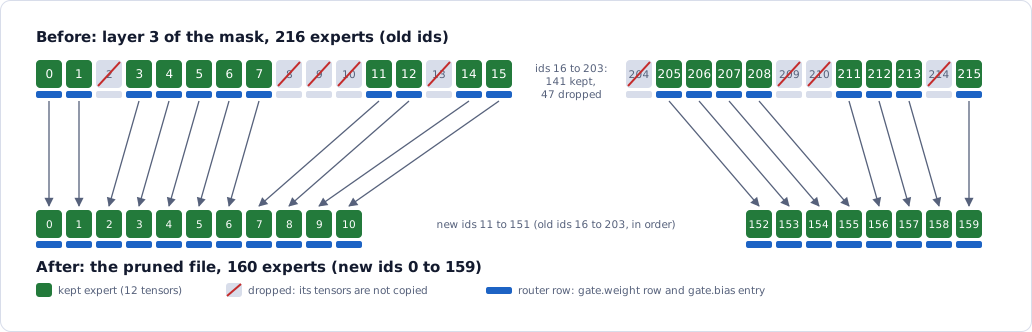
New ids for the kept experts, from the real keep map of layer 3. The kept ids keep their ascending order and close the gaps: old 3 becomes new 2, old 11 becomes new 7, and old 215 becomes new 159. The router row of each expert (blue bar) moves with it, so the router still scores the same experts. The tool applied one keep map per layer to all 43 layers.
The tool also set the expert count to 160 in config.json and quantization_config.json, because vLLM stops at load if the counts do not match. It also rewrote the weight index and the manifest, which the server checks at every boot.
The build
A script ran the tool in a container, with the stock folder mounted read-only.
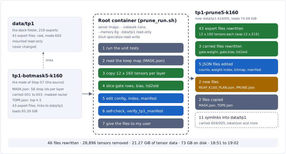
The prune tool. The mask folder held only new router files and links to the stock expert files, so the tool read the expert bytes from the stock folder. Green files hold changed tensor data, and blue JSON files hold new counts and checksums. The dashed box holds the files that did not change: they stayed links.
The build ran on 2026-11-06 and took about 11 minutes. It rewrote 46 files: the 43 expert files and the 3 files with the router tensors. It removed 28,896 tensors (43 layers × 56 experts × 12 tensors), or 21.27 GiB of tensor data.
The self-check
A rewrite of this size had to be exact. At the end of the build, the tool read the new folder and the source again. It confirmed that all 82,560 kept expert tensors and the 5,463 other tensors were byte-equal to the source. It also confirmed that the router tensors and tid2eid followed the new ids, and that the manifest matched every file.
The self-check passed on the first build.
Test boot of the pruned model
The pruned model had one job: to behave exactly like the mask, with the same replay result and the same speed. It needed no new full runs or final review, because the mask had already passed them. On 2026-11-06, a script stopped my live server and booted the pruned model with the stock draft model. It ran the replay screen and the two speed tests, and then it restored the live server.
| Stock model | Mask (the pick) | Pruned model | |
|---|---|---|---|
| Weights loaded | 95.39 GiB | 95.39 GiB | 74.09 GiB |
| Replay NLL change | 0 | +2.27% | +1.89% |
| Tool names | 77 of 83 | 79 of 83 | 78 of 83 |
| Bot test | 33.64 tok/s | 33.98 tok/s | 33.13 tok/s |
| Code test | 38.86 tok/s | 42.07 tok/s | 40.10 tok/s |
| KV cache | 7.36 GiB (269,629 tokens) | – | 29.76 GiB (1,089,707 tokens) |
21.30 GiB less memory. vLLM printed “Model loading took 74.09 GiB”, against 95.39 GiB for the stock model. My estimate from the exact tensor sizes was 74.1 GiB. My cap was about 72 GiB, to leave room for the second model, so the pruned model was 2.09 GiB over it.
The same routing. The pruned model passed the replay screen at +1.89%, even 0.38% lower than the mask. That difference was only 0.15 points over the 0.23% noise floor, and in the better direction. A wrong expert map would have made the NLL clearly worse: the failed masks cost +3% to +6%.
The same speed. Both speed tests were inside the 4.2% noise of the stock model: −1.5% in the bot test and +3.2% in the code test. The code test was 4.7% slower than the mask, due to one trial.
The freed memory went to the KV cache. I kept GPU_MEMORY_UTILIZATION at 0.93, so vLLM filled the same memory budget as before. It gave all of the freed memory to the KV cache, which grew from 7.36 GiB to 29.76 GiB: about 4 times as many tokens.
Deploy and pin the KV cache
I deployed the pruned model on 2026-11-06, and I kept the stock server intact for a rollback.
After the deploy, the KV cache took the memory that the prune freed: 29.8 GiB, room for 1,091,301 tokens. The whole machine had only 2.4 GB left. My bot did not need a cache that large, and the second model needed that memory.
The first try: a lower memory budget
My first idea was a lower GPU_MEMORY_UTILIZATION, the share of the 121.7 GiB that vLLM may use. A test boot at 0.73 failed: only 5.82 GiB was left for the KV cache, and vLLM needs room for at least one request of the full context length (6.54 GiB at 128k). A shorter context saved too little, so I kept the 256k context and looked for a different control.
The fix: set the KV cache size directly
I added --kv-cache-memory-bytes 8589934592 to the server flags. vLLM then reserved exactly 8 GiB for the KV cache and skipped its own memory estimate.
| After the deploy | After the pin | |
|---|---|---|
| KV cache | 29.8 GiB | 8 GiB |
| KV cache tokens | 1,091,301 | 292,952 |
| Memory used on the machine | 120.6 GB | 100.9 GB |
| Memory available | 2.4 GB | 23.7 GB |
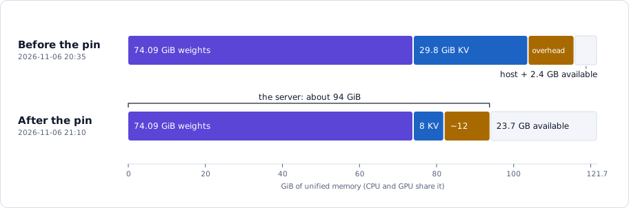
The live server before and after --kv-cache-memory-bytes. Only the KV cache changed: 29.8 GiB became 8 GiB. The weights stayed at 74.09 GiB, and the runtime overhead (draft model, activations, CUDA graphs, non-torch memory) was about 12 GiB after the pin.
8 GiB was enough for my bot. Its largest session was about 100k tokens, and the 292,952 tokens held 1.14 requests of the full 256k context.
A new draft model
The pruned model still used the stock DSpark draft.
Why a new draft model
The DSpark draft had its own MTP layer with 64 of the 216 experts. The stock draft chose those 64 by the public REAP rank, and that was a poor fit for my bot. Only 16 of the 64 were among my bot’s 64 most used experts in layer 42, and those top 64 carried 68% of the routing weight.
Instead, I built a new draft model, dspark-draft-k64-bot. It kept the 64 MTP experts with the highest bot rank in layer 42. It had the same size as the stock draft model, 3.0 GB.
Results
On 2026-11-07, a script booted the live pruned model with the new draft model and ran both speed tests. Then it restored the live server.
| Speed test | Stock draft model | Bot-rank draft model | Speed change | Acceptance change |
|---|---|---|---|---|
| Bot test | 33.13 tok/s, 2.05 per draft | 34.50 tok/s, 2.14 per draft | +4.1% | +4.7% |
| Code test | 40.10 tok/s, 2.52 per draft | 40.69 tok/s, 2.61 per draft | +1.5% | +3.5% |
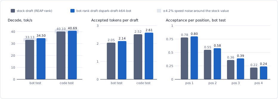
The draft test of 2026-11-07, on the live pruned model. Left: the bot gain (+4.1%) is just inside the grey noise band, and the code gain (+1.5%) is well inside it. Middle and right: the acceptance rose in both tests and at every draft position.
A small gain, just inside the noise. The bot test gained 1.37 tok/s, just under the 4.2% noise floor (1.42 tok/s). The code test gain was well inside the noise. My own rule said that a change counted only above the noise, so by that rule, the new draft model did not qualify.
But the gain was most likely real. Both tests moved in the same direction. The acceptance also rose at every draft position. The right panel shows the share of drafts in which the target model accepted the token at each position. It rose from 0.78 to 0.80 at position 1, and from 0.22 to 0.24 at position 4.
And the new draft model cost nothing. The switch was one mount line in the compose file and a short reboot.
So I switched to the bot-rank draft model on 2026-11-07. The server came back with the same 74.09 GiB of weights and 292,952 KV cache tokens.
The final memory savings
I removed 56 of the 216 routed experts in each layer, and I cut the experts per token from 6 to 5. Here is the stock model next to the live model of today:
| Stock model | Pruned model, live | |
|---|---|---|
| Routed experts per layer (K) | 216 | 160 |
| Experts per token (top-k) | 6 | 5 |
| Weights loaded | 95.39 GiB | 74.09 GiB (−21.30 GiB) |
| KV cache | 7.36 GiB (269,629 tokens) | 8 GiB, pinned (292,952 tokens) |
| Replay NLL change | 0 | +1.89% |
| Bot test | 33.64 tok/s | 34.50 tok/s |
| Code test | 38.86 tok/s | 40.69 tok/s |
When I started, only 4 GiB stayed free with the stock model loaded. Now the whole server uses about 94 GiB, and 23.7 GB of host memory stays available. The bot showed no loss that I noticed, and the decode speed stayed the same or got faster.
That memory is for the second model of my router. The host (the OS, the gateway, a browser and the CLIs) needs about 5 GiB, and I also want a free margin. That leaves about 12 GiB for the second model with a 10 GiB margin, or about 18 GiB with a 4 GiB margin.
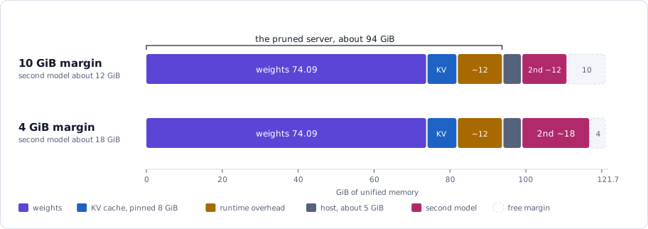
The room for a second model, drawn to scale, with two sizes of free margin. The share of the second model must hold its weights, its KV cache and its CUDA graphs. The values are estimates, and a boot with two models will measure the real ones.
This is less than the 22 GiB that my first plan assumed, for two reasons. The pruned model is 2.09 GiB over my 72 GiB cap, and the live server needs more runtime memory than its boot profile showed. So an MoE model or a small dense model now fits better than a 4-bit 27B dense model.
The biggest lessons
- A public expert rank is not your traffic. The REAP rank failed at K 192 (+3.31%). The rank from my bot’s own traffic cost only +0.29% at K 176. Rank the experts on the traffic that the model will serve.
- Test with a mask before you rewrite any weights. The mask hid experts from the router with a bias of −1e4, and it took about a minute to build. The pruned model then matched the mask within the noise.
- K saves memory, and top-k saves time. K 160 at top-k 6 decoded 6.4% slower in the bot test, because each token still ran 6 experts. Top-k 5 won the speed back, and top-k 4 cost too much quality (+6.05%).
- A pruned model needs a new look at its draft model. The mask lowered the bot acceptance from 2.25 to 2.09. A draft model ranked on my bot’s traffic won part of it back (+4.7%).
- Measure the noise floor before you read a result. Two runs of the same model differed by 0.23% in NLL and 4.2% in speed. Without those numbers, I could not have read the test boot or the draft test.
- Check the LLM judge with controls. Three runs of the stock model against itself gave no significant result. Only then did 44 wins and 19 losses mean “no loss”.
- Pin the KV cache when two models share memory. vLLM gives all of its free budget to the KV cache. The flag
--kv-cache-memory-bytesfixed it at 8 GiB and freed 21.3 GB of host memory.
Thanks for reading! I will continue to find interesting ways to prune and optimize my local models. If you have any questions or suggestions, feel free to reach out.
My code is in this repo: czhou578/dsv4-specialize. Its “Files” section lists the weight tools, the expert capture, the test boots and the run scripts of this post.
The tool that built the bot-rank draft model is in the server repo: build_dspark_draft.py.
The eval harness (the replay screen, the speed tests, the full runs and the LLM judge) is in my bot’s repo, which is private.
CZ